Crowdsourcing Inflationary Expectations through Text Mining: Do the Pink Papers whisper or talk loudly?
Ashok Banerjee , Ayush Kanodia , Partha Ray Download Article
How do we know about the general sentiment in the economy? Is it bullish or bearish? This question seems to haunt academicians and policy makers alike. The best way to gauge it is perhaps approaching the public. The general philosophy is best captured in the burden of Kishore Kumar’s song of Rajesh Khanna starrer movie Roti (1974) that goes, “Yeh jo Public hai – sab jaanti hai“. The question is: where does one meet the public and how does one listen? Does the public whisper or talk loudly? More importantly, does one get a unified message from such public talk or does all information get drowned in cacophony? This paper makes a preliminary attempt to gauge public opinion in newspaper reports. Within this general philosophy, our attempt in this paper is, of course, more modest. We look into one particular economic variable, viz., inflation.
Needless to say, Inflationary expectations tend to play a crucial role in macroeconomic and financial decision / policy making. In particular, it is of paramount importance when monetary policy is conducted within an inflation targeting framework or when the financial market player is thinking of her return from the bond / forex markets. But a perennial question in this context is: how to measure inflationary expectations? Three broad strands are identified in the literature. First, model based forecasts (univariate or multivariate variety) are often taken recourse to. Second, inflationary expectations are also derived from class / group-specific inflationary expectations surveys routinely conducted by central banks / financial data providers. Third, inflationary expectations / perceptions are also inferred from the market yields of inflation-indexed bonds.
While each of these methods is useful, each has its limitations as well. In this paper we propose and adopt a novel method of inferring inflationary expectations using a machine learning algorithm by sourcing economic news from the leading financial dailies of India. In particular, we argue that Economics / Finance can leverage advances in artificial intelligence (AI), natural language processing (NLP) and big data processing to gain valuable insights into the potential fluctuations of key macro indicators and attempt to predict the direction (upward versus downward) of monthly consumer price inflation.
The remainder of this article is organized as follows. While section 2 discusses the motivation of this approach, the methodology is delved in section 3. Section 4 presents the results and section 5 concludes.
- Motivation and Received Literature
The motivation of this approach can be traced in two distinct strands of literature. First, among the monetary economists there is a large literature of what has come to be known as the “narrative approach to monetary policy”. While the origin of this approach can perhaps be traced to Friedman & Schwartz (1972)’s Monetary History of United States, Boschen and Mills (1995) derived an index of monetary policy tightness and studied the relation between narrative‐based indicators of monetary policy and money market indicators of monetary policy. They found, “Changes in monetary policy, as measured by the narrative‐based policy indices, are associated with persistent changes in the levels of M2 and the monetary base”. More recently, Romer and Romer (2004) derived a measure of monetary policy shocks for the US. Instead of taking any particular policy as an indicator of monetary policy shock, Romer and Romer (2004) derived a series on intended funds rate changes around meetings of the Federal Open Market Committee (FOMC) for the period 1969–1996 by combining the “information on the Federal Reserve’s expected funds rate derived from the Weekly Report of the Manager of Open Market Operations with detailed readings of the Federal Reserve’s narrative accounts of each FOMC meeting”. But all these papers involve some degree of subjectivity of reading the policy narratives. Hence a key question remains: how does one get rid of this subjectivity? It is here that more contemporary tools of machine learning, nature language and big data processing become helpful.
This second strand of literature comes from machine learning. To get a perspective of its emergence, it is important to note that there has been a healthy scepticism and conscious efforts on the part of the academics to avoid forecasting economic / financial variables. Smith (2018) in a recent article attacked the profession and went on to say:
“Academic economists will give varying explanations for why they don’t pay much attention to forecasting, but the core reason is that it’s very, very hard to do. Unlike weather, where Doppler radar and other technology gathers fine-grained details on air currents, humidity and temperature, macroeconomics is traditionally limited to a few noisy variables …. collected only at low frequencies and whose very definitions rely on a number of questionable assumptions. And unlike weather, where models are underpinned by laws of physics good enough to land astronauts on the moon, macroeconomics has only a patchy, poor understanding of individual human behavior. Even the most modern macro models, supposedly based on the actions of individual actors, typically forecast the economy no better than ultra-simple models with only one equation ….whatever the reason, the field of macroeconomic forecasting is now exclusively the domain of central bankers, government workers and private-sector economists and consultants. But academics should try to get back in the game, because a powerful new tool is available that might be a game-changer. That tool is machine learning” (emphasis added).
But what is machine learning? Loosely speaking, “Machine learning refers to a collection of algorithmic methods that focus on predicting things as accurately as possible instead of modelling them precisely” (Smith, 2018). With rapid advances in storing and analysing large amounts of unstructured data, there is increasing awareness that these data could be a rich source of useful information for assessing economic trends. Various attempts have emanated in forecasting macroeconomic and financial variables. Illustratively, Nyman and others (2016) used the Thomson‐Reuters News archive (consisting of over 17 million English news articles) to assess macroeconomic trends in the UK. More recently, using machine learning techniques Shapiro & others (2018) developed new time series measures of economic sentiment based on computational text analysis of economic and financial newspaper articles from January 1980 to April 2015. There is now a burgeoning literature on this issue, thanks to the Rational Expectations thinking that policy making needs to have some sense of the future sentiment / expectations. However, the policy maker needs to take care of the popular adage of Goodhart’s law whereby “when a measure becomes the target, it can no longer be used as the measure”, so that forecasts fail when used for policy prescription and when used as targets naively.
Detection of sentiment from the newspapers seems to be less prone to this syndrome. Much of this literature asks the machine to find out the recurrence of some key words with appropriate identifiers in the newspaper articles so that the detection does not get corrupted by any subjective bias. Our paper ties to decipher the inflationary sentiment from the newspaper articles.
- Methodology
Literature on sentiment analysis shows that mere frequency of information arrival (news articles) may not explain change in an economic variable. What drives economic agents is the sentiments (i.e., quality) of information. Extracting sentiment from newspaper reports is one of the major contributions of our paper.
We develop a system over python and several accompanying libraries to access large chunks of newspaper data, parse and process the news content, and make a well founded estimate of the direction of inflation (CPI) in the near (next) month using sentiments generated from news content for the current month.
Input: To forecast inflation for a month (released in the middle of the month), we take as input news from 20th of previous month to 10th of current month. We can take as many newspapers as we like. For instance, for inflation of April 2015 (released an Apr 15), we use news from March 20th 2015 to April 10th 2015. Note that CPI numbers are released in the middle of a month (12th to 18th).
Output: For each month, we consume all the input news content and after processing, produce a single number which denotes the sentiment towards inflation for that month.
Component: Our system consists of the following components arranged in a pipeline.
Figure 1: System pipeline
|
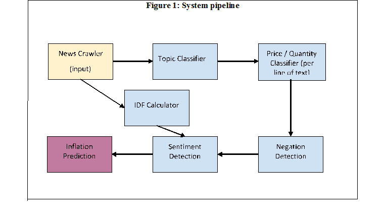
Our search is limited to news from two business dailies (Economic Times and Business Line). We crawl the news from the “factiva” database online using a python tool. This is our input to the rest of the system.[1] Let us now turn to each of the components of Figure 1.
Topic Classifier
This module takes as input a news article and classifies it into one of the sub baskets used to calculate the overall CPI. The sub baskets are fuel, food, cloth, housing, intoxicants (alcohol and various tobacco consumables) and miscellaneous.[2] The classifier can classify an article into one of these multiple baskets. We manually labelled about 4000 articles for two random months (Nov-Dec 2015 and 2016) to serve as our training set. It is interesting to note that the training dataset included the period of demonetisation.
Price/Quantity Classifier (Per line of text)
This module takes as input a line of text from an article and flags it as talking of price of the commodity, quantity of the commodity, of both, or of neither. Each line is classified into one of four categories – talking of neither price or production, of only price or only production, or both. The idea is that inflation expectation is triggered by knowledge of either demand pull inflation (higher prices due to higher demand) or cost push inflation (higher prices due to lower supply).
For instance, “Oil prices unlikely to rise” would be classified as talking of only price, “OPEC cuts output on breakdown of talks” would be classified as talking of only production, “While prices seem to be rising, production is not falling commensurately, leading to inventory accumulation” would be classified as talking of both price and production, while “New policies on the horizon” would be classified as talking of neither price nor production.
Negation Detection (Per line of text)
This module takes as input a line of news text and checks whether parts of the line are negated using negation words as “not”, “unlikely”, “improbable” etc. The way it does this is as follows. For example, consider the line: “Oil prices not likely to rise”. The negation detector returns as output “Oil prices <negated scope> not likely to rise <\negated scope>”. The additional markers inform us of the part of the sentence whose adjectives (in this case rise) are negated in meaning. This is utilised downstream in sentiment detection (see example in later section on sentiment detection).
IDF (Inverse Document Frequency) Calculator
TF (Term Frequency) of a word is defined as the number of times a word is seen in an article (document). IDF of a word is defined as a measure of the salience (or contribution to new information) of a word, based on how likely the word is to appear as a prior. If we merely use Term Frequency, we would not account for the fact that words which have a high prior of occurring will bias our estimate. For instance, determiners like a, the, will have naturally high TF, and they need to be downweighted.
This module looks at sentiment words (generally adjectives) which we use downstream to infer sentiment from news articles, and calculates their IDF (Inverse Document Frequency) over our news articles dataset. Hence, for a word which appears in every document, IDF is zero, whereas it is most for a term which occurs in only one document.
Our IDF is calculated based on the news articles for the first six months of our dataset (months of July-December 2015). This should have broad enough coverage to give us a principled and correct estimate of IDF.
Sentiment Detection
This module takes as input an article, and rates each line of text in the article with a number which describes whether the line indicates a rise or a fall in inflation. For this, it uses the information inferred upstream – whether the line talks about price/production, its negated scopes, and the relative strengths of sentiment adjectives. Sentiment adjectives which appear closer to the mentions of price/production are weighted more.
Illustratively, consider the sentence “Oil prices not likely to rise”. As explained earlier, this sentence is classified as talking of price (due to the word “prices”). Consider the IDF of rise to be 2.0. Consider the dampening factor for interword separation between the adjective (rise)and subject (prices)to be 0.8. We exponentiate the dampening factor to the number of words in between, which is 3 in this instance(not likely to). Therefore, our sentiment score is (0.8^3)*2=1.024. However, the sentence adjectives are negated as determined by the output of the Negation Detection module (“Oil prices <negated scope> not likely to rise <\negated scope>”). Therefore, the value for rise is negated to -2.0, and we end up with a sentiment score of -1.024
After scoring each line, the article sentiment score is simply a weighted sum of the scores for the individual lines. It strongly attributes more weight to the headline and line towards the beginning of the article. This method provides an unscaled number (which takes all real values, but is likely in the range (-10, 10) which determines the strength (and direction) of sentiment of each line in the article. We dampen this unscaled number to a number between (0, 1) (exclusive), using a dampening function function. The higher the number, the more it indicates a positive sentiment towards a rise in inflation.
Inflation Prediction
We follow a short-term prediction approach with monthly updation of parameters. We use individual sentiment values for each article in a month, and aggregates them into a single predicted inflation number for the next month.
We learn a multivariate regression model over our training months, which is as follows:
I (t) = k + aSfood (t – 1) + bSfuel (t – 1) + cScloth (t – 1) + dSmisc (t – 1) + eSgeneral (t – 1) + fIdm
is an indicator variable which is 0 for all months before demonetization and 1 afterwards. This is to inform the model that an external event, which affects public sentiment strongly, has occurred. We note that the introduction of this variable results into a significant improvement in our prediction model. We may introduce such variables for other similar external shocks to the economy, which strongly affect inflation. is Inflation at time t (month t), and is sentiment for basket ‘x’.
We predict inflation for month i, using the sentiments and inflation figures of month i – 1. Similarly, for month i + 1, we use the actual inflation number for month i, so that our model is improved.
Input Size
Per newspaper, there are about 50 articles per day. That adds up to 1500 articles per month per newspaper. We currently work with two newspapers (Economic Times and Business Line), therefore we have around 3000 articles per month (Table 1).
| Table 1: Summary statistics for number of articles in each component of CPI | ||||
| Topic | Mean | Median | Min | Max |
| Fuel | 108 | 100 | 38 | 234 |
| Food | 149 | 138 | 94 | 239 |
| Cloth | 30 | 29 | 13 | 48 |
| House | 71 | 73 | 40 | 132 |
| Pan and intoxicants | 6 | 6 | 1 | 15 |
| Miscellaneous | 337 | 338 | 236 | 446 |
| General | 6 | 5 | 0 | 22 |
Each sub basket component of CPI has about 5 – 400 articles per month. The general category is not a CPI component, but we measure sentiment as belonging to this category if an article directly addresses inflation (and does not talk of any of the subcomponents of the CPI basket). This serves as a useful signal to measure sentiment towards overall inflation.
As a rough estimate, misc contains the most number of articles per month at 350 – 400 on average, and the other baskets contain 50 – 250 articles per month on average. There are very few articles (about 7 on average) per month addressing the general category.
- Performance Metrics and Results
It takes about 60 – 120 seconds of real time on a commodity PC to process an entire month’s news and output the sentiment score for the month. The configuration used is an i5 2.30 GHz processor, with 2 cores and 2 threads per core (although at present we do not use multithreading). Our system is built in python and these measurements were made on Linux. We should note that this is unoptimized code, so within python itself, optimizing should lead to faster performance. Further, using a lower level language and libraries should lead to even faster performance. There is great scope for parallelization in our system, since each article is processed independently of the other. Leveraging this could lead to orders of magnitudes improvements too.
We calculated monthly sentiment for each of the CPI baskets and performed a univariate regression of basket sentiment on basket inflation. We found high univariate correlation for the food, fuel, cloth and misc baskets, as well as high correlation between sentiment for the general category and overall inflation. The results are given in Table 2.
| Table 2: Univariate Regressions of each components of CPI
(General form: Ii(t) = k + a Si(t-1); for i = food, fuel, cloth, misc, general) |
|||||
| coefficient | coefficient values | Standard errors | t_values | probabilities | |
| Food | k | 0.43 | 1.07 | 0.40 | 0.69 |
| a | 0.4797 | 0.068 | 7.099 | 0.0 | |
| Fuel | k | 2.44 | 0.598 | 4.076 | 0.0 |
| a | 0.2326 | 0.040 | 5.842 | 0.0 | |
| Cloth | k | 5.25 | 0.720 | 7.29 | 0.00 |
| a | 0.8382 | 0.25 | 3.42 | 0.00 | |
| Misc | k | 2.40 | 0.75 | 3.187 | 0.002 |
| a | 0.16 | 0.041 | 3.801 | 0.00 | |
| General | k | 5.17 | 0.51 | 10.11 | 0.00 |
| a | 0.42 | 0.17 | 3.56 | 0.001 | |
Further, the multiple regression leads to a high significance for fuel, food as well as general sentiments. Table 3 reports the regression results.
I (t) = k + aSfood (t – 1) + bSfuel (t – 1) + cScloth (t – 1) + dSmisc (t – 1) + eSgeneral (t – 1) + fIdm
| Table 3: Projecting General CPI Inflation: Base line Regression | ||||
| coefficient | coefficient values | Standard errors | t_values | probabilities |
| k | 2.1106 | 0.849 | 2.486 | 0.015 |
| a | 0.0848 | 0.041 | 2.071 | 0.042 |
| b | 0.2377 | 0.048 | 5 | 0 |
| c | 0.176 | 0.179 | 0.986 | 0.328 |
| d | -0.0588 | 0.051 | -1.147 | 0.255 |
| e | 0.1697 | 0.084 | 2.023 | 0.047 |
| f | -2.2455 | 0.463 | -4.851 | 0 |
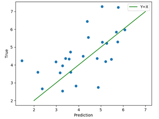
Prediction Results
How is the predictive performance of the model we have developed? The figure below charts a scatter plot of true inflation versus predicted inflation using our model. We achieve a correlation score of 0.59.
| Figure 2: Inflation (True versus Predicted) |
 |
- Concluding Observations
Measuring inflation expectation is a key component of economic and financial policy making. We use text mining to predict inflation expectations. This experiment of investigating whether inflation perception can be measured using newspaper text essentially consists of two sub experiments. The first is to check how well an automated system, when invoked on a single newspaper article, can infer its general sentiment about inflation. This is to say that if an expert (economist) were to read the same article and conclude that this article says price is going to rise, the system should be able to provide the same result. The second is to check whether given such sentiments about each article, does the aggregated sentiment from the monthly news remain significant and relevant to predict actual inflation numbers.
The first of these subtasks, we must say, has achieved high accuracy. When we evaluated the sentiment inferred by the system on individual articles by hand, the system performed accurately almost all the time, and even corrected the human labeller on some occasions! To this extent we believe that the underlying Natural Language Processing used to generate such sentiment may not benefit much from improvements, as our “simple” model appears to do well. The most significant way to improve this now could be to target a finer level of granularity in terms of inferring article sentiment. That is to say, the challenge is to build a system which not only tells us whether price is going to rise or fall, but also by how much. Note that this task is indeed hard for even an expert to complete.
The second of these subtasks however, may see various improvements. For one, we have yet only observed (largely) direction of sentiment of an article. However, if the article talks about something relatively unimportant, we may wish to discount its contribution to overall sentiment. This may be based on the commodity it is talking about, its source, the tense of the text, and the timing of the article (within our prediction horizon which is monthly), none of which we have yet included in our model. Future work in this direction may aim to incorporate such factors.
One of the principled limitations of our approach is that in a developing country like India (versus say, the United States), financial news often does not percolate (fast enough) to the rural population. Hence, using only financial news sentiment to measure perception towards inflation may not be good enough. To this end, we performed our predictions (as above) on urban inflation instead of overall inflation, and saw a slight improvement in results.
Of course, one of the crude ways to improve our system further would be to use more newspapers, and to use more labelled data. We could also include other measures of public sentiment for inflation, in the form of well-read blogs, news published by the central bank in press releases, and even social media data such as twitter posts.
This is a novel, if not the first attempt, to quantify public sentiment towards inflation by inferring it from newspaper text for India. Besides, it compares well with the IESH (Inflation Expectation Survey of Households) conducted by the RBI in order to measure inflation perception as IESH achieves a correlation coefficient of 0.50 in predicting the actual inflation figure, whereas we obtain 0.59 with our method. We hope that such approaches to predicting macroeconomic variables are investigated further by the research community, and fruitful results applied in public policy making.
References
Boschen J. and S. Mills (1995): “The relation between narrative and money market indicators of monetary policy”, Economic inquiry, January, pp 24-44.
Friedman, Milton and Anna J Schwartz (1972): A Monetary History of United States, 1867 – 1960, Princeton: Princeton University Press.
Nyman, Rickard , David Gregory, Sujit Kapadia, Paul Ormerod, David Tuckett & Robert Smith (2016): “News and narratives in financial systems: Exploiting big data for systemic risk assessment”, Bank of England Working Paper No. 704.
Romer, Christina D. And David H. Romer (2004): “A New Measure of Monetary Shocks: Derivation and Implications”, American Economic Review, September, 94(4): 1054 – 1083.
Shapiro, Adam Hale, Moritz Sudhof, and Daniel Wilson (2018): “Measuring News Sentiment”. Federal Reserve Bank of San Francisco Working Paper, available at https://doi.org/10.24148/wp2017-01
Smith, Noah (2018): “Want a Recession Forecast: Ask a Machine”, Bloomberg, May 13, 2018, available at https://www.bloomberg.com/view/articles/2018-05-11/want-a-recession-forecast-ask-a-machine-instead-of-an-economist
[1] We are in the process of extending it to use news from “Business Standard” and “Financial Express”.
[2] The relevant weights for each of these groups are 45.86%, 2.38%, 6.53%, 10.07%, 6.84%, and 28.32%, receptively.