Each year in April and October, the International Monetary Fund (IMF) comes up with two of its flagship publications, viz., the World Economic Outlook (WEO), and the Global Financial Stability Report (GFSR), coinciding with the Spring and the Annual Meetings of the IMF. While the WEO is a product of the Research Department of the IMF, the GFSR is coordinated by the Monetary and Capital Markets (MCM) Department. Often in the media attention on the WEO, the coverage of the GFSR gets somewhat lost, perhaps unjustifiably. The recent GFSR, which was published on October 18, 2019, is an outstanding report with rich analytical content as well as well-informed market perception. Spanning over seven chapters and covering issues as diverse as, global corporate vulnerabilities, institutional investors, emerging and frontier market, banks’ dollar funding, and sustainable finance, the report does justice both to the depth and the breadth of these issues. Many of these issues are beyond the scope of the current commentary. Instead, the present article looks into some fault lines of contemporary global financial stability, as revealed in the current GFSR.

Major Fault Lines

At the risk of presenting broad generalizations, a look at the current trends of global financial markets reveal the following six broad trends:

1. In the backdrop of the US-China tariff war, there has been significant weakening of business sentiments.
2. Coupled with technology and geopolitical tensions, such erosion of business sentiments have led to increases in policy uncertainty.
3. This is perhaps best reflected in pronounced decline of long-term yield, which is largely seen as a leading indicator of a possible slowdown.
4. However, the equity market has shown some sort of irrational exuberance despite the low business mood.
5. The key to understanding the contradiction between the bond and equity markets can perhaps be traced in a shift toward “a more dovish monetary policy stance across the globe”. In particular, the futures markets tend to indicate that monetary policy rates are expected to be lower for “longer than anticipated at the beginning of the year”.
6. There has been huge increases in debt stock and a significant portion of outstanding debt stock are at negative

While all these trends seem to have profound implications for global stability, in specific terms this commentary points out to three major traits of the current global financial condition, as highlighted in the GFSR.

Swings in Financial Markets

Global financial markets exhibited significant swings in recent period, reflecting interplay of two policy sources, viz., imposition of tariff on the part of the US on China, on the one hand, and the US monetary policy actions (both actions as well as intended), on the other (Chart 1). For example, there has been significant fall in global equity prices, after US President Trump’s speech of May 29, 2018 when he categorically mentioned, “China has consistently taken advantage of the American economy with practices that undermine fair and reciprocal trade” (Chart 1.1).[1] On the other hand, advanced economies governments’ bond yields of various maturities have experienced significant declines since October 2018. Of course, after converging to very low levels, in recent past there has been some increase (Chart 1.3).

Chart 1: Global Financial Markets
1.1   World Equity Prices (Index: Jan. 1, 2018 = 100)	1.2   Option-Implied Volatilities in the US Equity and Treasury Bond Markets (Indices)
1.3    Advanced Economy Government Bond Yields	1.4   Advanced Economy Government Bonds (Percent of bonds outstanding, by yield)
Source: Global Financial Stability Report, IMF, October 2019.

In consonance with the gyrations in the financial markets, there has been substantial increase in volatility as reveled by movements in option-implied volatilities in the US Equity and Treasury Bond Markets (Chart 1.2). Finally, along with flattening (and in some case inverting) of the yield curves, the amount of bonds with negative yields has increased to about $15 trillion, “including more than $7 trillion in government bonds from large advanced economies, or 30 percent of the outstanding stock” (Chart 1.4).

Mr Powell versus Mr Trump: The Good Cop – Bad Cop Syndrome?

While the report is couched in the usual politically correct and conservative language of the IMF, there is a theme of the destabilizing effect of the tariff war and the stabilizing effect of the US monetary policy, running underneath the report. All actions / speeches of the US Fed Chairman have typically been followed up an upbeat mood in financial markets. Illustratively, after the US Fed Chairman, Mr Jerome Powell spoke on “Economic Outlook and Monetary Policy Review”, on June 25, 2019 at the Council on Foreign Relations, New York, the world equity prices increased significantly and volatility reduced.  Interestingly, instead of announcing any tangible policy decisions, he went to say:

“We did not change the setting for our main policy tool ….but we did make significant changes in our policy statement. Since the beginning of the year, we had been taking a patient stance toward assessing the need for any policy change. We now state that the Committee will closely monitor the implications of incoming information for the economic outlook and will act as appropriate to sustain the expansion, with a strong labor market and inflation near its symmetric 2 percent objective”.[2]

Does this mean the global uncertainties created by the trade and technology war between the US and China be countered solely by the arsenal of monetary policy? The answer at best is still couched in mystery. Interestingly, all the major   central banks have adopted an easy money stance in 2019 (Chart 2). Significantly three major central banks, viz., Japan, Euro Area and Switzerland have negative policy rates; these are expected to continue at least for next three years.  In some cases, the extent of negative interest rates has got accentuated. Illustratively, on September 12, 2019, the European Central Bank reduced the interest rate on its deposit facility by 10 basis points to (-) 0.50 per cent.[3]

Are the expectations from monetary policy too much? Can the negative effects of a trade war be countered by an overtly accommodative monetary policy?  Does monetary policy has Atlas-like quality and has been condemned to hold up the celestial heavens for eternity? All these questions assume importance. In fact, a case in point is the recent spat between President Trump and Fed Chairman Powell. Reportedly, Mr. Trump called the US  monetary policy “insane” and added that Mario Draghi, President of the European Central Bank, should take the helm instead (Financial Times, June 26, 2019).

Chart 2: Actual and Expected Monetary Policy Rates in Advanced Countries (Percent)

E: Estimate Source: Global Financial Stability Report, IMF, October 2019.

Build-up of Financial Vulnerabilities

Accommodative monetary policy has its limitation. GFSR made a detailed sectoral and country-specific analysis of financial vulnerabilities and noted, “The prolonged period of accommodative financial conditions has pushed investors to search for yield, creating an environment conducive to a buildup of vulnerabilities.” Chart 1 below reports the financial vulnerabilities for six specific sectors, viz., banks, households, non-financial firms, Sovereigns, other non-bank financials, and insurers. Vulnerabilities of other non-bank financial entities seem to have increased since April 2019. In particular, among other nonbank financial entities, “vulnerabilities are high in 80 percent of economies with systemically important financial sectors, by GDP” and at a level that was attained during the global financial crisis. This could be due to an increase in leverage and credit exposures in the US and the Euro Area where institutional investors, in their quest for maximizing yield and targeted return, could have taken on riskier positions.

Chart 1: Global Financial Vulnerabilities: Proportion of Systemically Important Economies with Elevated Vulnerabilities, by Sector

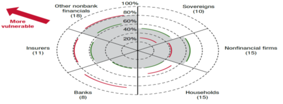
Source: Global Financial Stability Report, IMF, October 2019.

Concluding Observations

One of the lessons from the global financial crisis is perhaps that vulnerabilities get built during good times. We do not know whether the current situation when the threats of trade war looms large, and bond yields have gone to very low levels (perhaps indicating global slowdown) can be termed as good times. But, the burdens of rising corporate debt, increasing holdings of riskier and more illiquid assets by institutional investors, and external borrowing by emerging and frontier market economies may not be nullified by accommodative monetary policy alone. All these are omens in the apparent exuberance in select segments of global financial markets. Thus, in some sense the GFSR seems to be cautiously pessimistic and warn us about the bad old days to come.

[1] The speech was followed by a re-imposition of a 25 percent tariff on all steel imports (except from Argentina, Australia, Brazil, and South Korea) and a 10 percent tariff on all aluminium imports (except from Argentina and Australia).

[2] Available at https://www.federalreserve.gov/newsevents/speech/powell20190625a.htm

[3] The interest rate on the main refinancing operations and the rate on the marginal lending facility have, however, remained unchanged at their current levels of 0.00 per cent and 0.25 per cent, respectively.

On 4^th November, 2019, the Reserve Bank of India (RBI) revised the liquidity risk management framework for the Non-Banking Financial Companies (NBFCs) and Core Investment Companies (CICs). The guidelines earmarked the roles and responsibilities of NBFCs in managing their liquidity risks and implementing the Asset Liability Management (ALM) framework under normal as well as distressed liquidity market conditions. In the following paragraphs, the core components of the regulatory guidelines for liquidity risk management framework of NBFCs is discussed, along with their broad implications:

Governance of Liquidity Risk Management

The RBI regulatory guidelines placed significant emphasis on the governance of liquidity risk management by putting the responsibility for management of liquidity risk on (a) the Board of Directors, (b) Risk Management Committee, (c) Asset Liability Management Committee (ALCO) and (d) Asset Liability Management (ALM) Support Group. To further elaborate, first and foremost, the RBI guidelines placed the overall responsibility of managing the liquidity risk of NBFCs with their Boards, and in accordance, proposed that the Boards should decide the strategy, policy and procedures of the NBFCs as per the liquidity risk tolerance limits set by them.

Thereafter, the responsibility for evaluation of overall risks faced by the NBFCs including the liquidity risk was assigned with the Risk Management Committee, which would be comprised of the Chief Executive Officer (CEO), Managing Director (MD) and Heads of various risk divisions. In addition, the Asset-Liability Management Committee (ALCO) would be entrusted with the responsibility for adherence to risk tolerance limits as set by the Board as well as the implementation of the liquidity risk management strategy of the NBFC. As per the RBI directives, ALCO need to be comprised of top management of the NBFC, and would be responsible for making decisions on desired maturity profile and mix of incremental assets and liabilities, sale of assets as source of funding and overall structure and strategy of liquidity positions and liquidity risk management at each of the NBFC branch levels. Finally, the Asset Liability Management (ALM) Support Group would be consisting of operating staff to analyse, monitor and report the liquidity risk profile to the ALCO.

Product Pricing and Off-Balance Sheet Exposures Consistent With Liquidity Risk Tolerance

The RBI guideline emphasized the need for a NBFC to clearly articulate its liquidity risk tolerance which is consistent with its business strategy and product focus, such that it could identify, measure, monitor and control its liquidity risk in accordance with such risk tolerance and ensure sufficient liquidity during its daily operations, both under normal and stressed market conditions. In this regard, RBI urged the NBFCs to incorporate the liquidity costs and benefits in its internal product pricing mechanism and evaluate the trade-offs during the new product approval process for all of its product and services related business segments.

The guidelines further emphasized the need for careful evaluation of liquidity risks arising out of off-balance sheet exposures, contingent liabilities and Intra-group Transactions and Exposures (ITEs). In this regard, it was suggested that the NBFCs should develop a robust framework to estimate the cash flows arising from assets, liabilities and off-balance sheet items over appropriate time horizons, including the impact of risk exposures on account of Special Purpose Vehicles (SPVs), financial derivatives, guarantees and commitments on liquidity risk of NBFCs. In the same manner, the guidelines also suggested NBFCs to recognize likelihood of enhanced liquidity risks arising due to Intra-group Transactions and Exposures based on complexity, risk profile and scope of operations of companies affiliated to the business group. The greater scrutiny and heightened regulatory focus on Intra-group Transactions and Exposures (ITEs) of NBFCs could have emerged in the immediate aftermath of series of credit defaults by Infrastructure Leasing & Financial Services (IL&FS) Group of companies.

Introduction of Liquidity Coverage Ratio (LCR) for Liquidity Risk Management

In line with the Basel compliant norms for the banking sector, the RBI guideline mandated all Non-Deposit taking NBFCs with asset size of INR 100 billion and above, and all Deposit taking NBFCs to maintain a liquidity buffer in terms of Liquidity Coverage Ratio (LCR) to ensure that NBFCs have sufficient High Quality Liquid Assets (HQLA) to withstand any acute liquidity distress scenario lasting for 30 days. The LCR requirement would be binding on NBFCs from December 2020 onward, as the following progressive LCR requirements:

The Liquidity Coverage Ratio (LCR) is defined as the stock of High Quality Liquid Assets (HQLA) divided by the Total Net Cash Outflows over next 30 calendar days. HQLA refers to liquid assets, which can be easily converted into cash at close to its intrinsic value, or used as collateral to raise funding during a period of financial distress. Thus, the basic purpose of mandating the LCR requirement on the NBFCs is to ensure that NBFCs have adequate level of liquidity safeguards in the form of HQLA in order to meet its liquidity needs for a period of 30 calendar days, even under major market disruption scenarios.

As per the guidelines, HQLAs are required to be low credit and market risk instruments having low valuation uncertainty and pricing complexity, low correlation with valuation of risky assets and publicly listed on any recognized stock exchanges. Further, HQLAs are financial instruments with active and large secondary markets which have dedicated market makers, low level of market concentration and are likely to get benefited from flight to quality capital movements under situations of broad systemic crisis.

Assets such as cash, government securities and marketable securities which are assigned zero risk weight by banks under standardized approach for credit risk may be considered in the computation of HQLAs for a NBFC at their fair value without any haircut. However, for certain other securities such as Corporate Bonds, Commercial Papers and Common Equity shares, haircuts between 15% to 50% may be applicable, depending upon the risk weight by banks under standardised approach for credit risk, credit rating of the financial instrument and nature of liquidity in the traded market of the financial security during a relevant period of significant liquidity stress.

Diversified Funding Strategy and Contingency Funding Plan

Diversified funding strategy and Contingency Funding Plan (CFP) have been among the key focus areas of this RBI regulatory guideline for NBFC liquidity risk management. As per the RBI directives, the NBFCs are required to develop a funding strategy that is diversified across both source as well as tenor of funding, so that it can avoid over-dependency on a single source of funding. This is particularly important, as the NBFCs had been heavily dependent on Money Market Securities such as Commercial Papers (CP) or Certificate of Deposits (CD) for their funding requirements, thereby exposing themselves to significant liquidity risk factors emerging from Asset Liability mismatch particularly during distressed money market conditions.

In terms of Contingency Funding Plan (CFP), the NBFCs would be required to formulate contingency plans containing details of potential sources and estimated amounts of contingency funding, along with expected lead time required to raise additional funds under distressed liquidity conditions. Given the inherent uncertainty and significant volatility of the market conditions, NBFCs would require a robust stress testing framework to simulate short-term as well as longer-term NBFC-specific and systemic liquidity stress scenarios where in a wide range of assumptions about the strength of NBFC operating business, financial conditions and macro-economic factors could be taken into consideration. In future, it is plausible that NBFCs would require to engage in significant employee skill building and competency enhancement exercises for this purpose, either through in-house or externally supported training and management development programs conducted by academic experts and industry professionals in the banking domain.

Public Disclosure Requirements Related to Liquidity Position and Liquidity Risk Management

RBI mandated the NBFCs to publicly disclose the Liquidity Coverage Ratio (LCR) related details including the level of High Quality Liquid Assets (HQLA), and break-up of expected cash inflows and outflows over next 30 days on a quarterly basis to enable the market participants to make an informed decision about the quality of liquidity position of the NBFC, and the soundness of its liquidity risk management framework. The enhanced public disclosure requirements are likely to assist the Credit Rating Agencies (CRAs) in evaluating the credit instruments issued by the NBFCs, and enable the portfolio managers of the Asset Management Companies (AMCs) in making better investment decisions, thereby putting additional capital market induced disciplinary pressures and monitoring oversight on the NBFC Board as well as their Top Management.

Granular Maturity Profiling enabled by Robust Management Information System

The RBI guidelines have put down responsibilities on the NBFCs to develop a reliant Management Information System (MIS) which can provide timely and forward-looking information on the liquidity position of the NBFC and the Group to the Board and the ALCO, both under normal and stressed market scenarios, by capturing all possible sources of liquidity risks and gathering granular and time-sensitive information, particularly during stress events.

An important element of the granular, time-sensitive information is the granular maturity bucket, which can be used for maturity profiling to estimate cumulative surplus or deficit of funds at various maturity dates for measuring the future cash flows of NBFCs in different buckets. For example, the guidelines mandate the NBFCs to segregate the 1 to 30 day time bucket into granular buckets of 1 – 7 days, 8 – 14 days and 15 – 30 days. This is expected to enable the NBFCs to estimate their short-term liquidity requirements on the basis of their business projections and other commitments for planning purposes as well as monitor their short-term liquidity risk on a dynamic basis over next 1 day to 6 months. The guidelines also require the NBFCs to restrict the net cumulative negative mismatches in the maturity buckets of 1 – 7 days, 8 – 14 days and 15 – 30 days to a maximum of 10%, 10% and 20% of the cumulative cash outflows in the respective time buckets.

Liquidity Risk Monitoring Tools

The RBI guidelines have emphasized on three critical liquidity risk monitoring tools for the NBFCs: (a) The first measure would identify the level of concentration in the funding channel of the NBFC so that withdrawal of any dominant funding source does not pose as a major liquidity risk problem for the entity. (b) The second measure would identify the amount of available unencumbered assets which could be used as collateral to raise additional secured funding in secondary markets in the event of an unforeseen liquidity disruption event. (c) Finally, a high-frequency measure of market data would be adopted to monitor news and capture information related to financial leverage, shape of yield curve and even breach or penalty in respect of regulatory requirements to serve as early warning indicator for potential liquidity concerns for the NBFCs.

Summary of Causes and Consequences

The NBFC sector has recently witnessed a major liquidity turmoil, with potentially significant adverse cascading effects even for the real economic sector. Since the banks were already burdened with high level of Non-Performing Assets (NPAs), the credit growth required to boost the level of economic activity in the real sector was critically dependent on the shadow banking channels for financing the consumption demands of the retail consumers as well as the investment needs of the corporate entities, particularly in the real estate, infrastructure and consumer durables sector. Unfortunately, a series of credit defaults by the NBFCs beginning with Infrastructure Leasing & Financial Services (IL&FS) Group, and subsequently Dewan Housing Finance Limited (DHFL) and Altico Capital, triggered a major credit market disruption, which increasingly threatened to pose as a systemic risk factor both for the private consumption and corporate investments which are heavily dependent on NBFC financing channels. In turn, the slowdown in real economy along with asset quality deterioration in NBFC balance sheets would impact the core banking sector which had exposures to both the NBFCs as well as the consumer and corporate borrowing markets.

The RBI guidelines on the liquidity risk management framework of the NBFCs would serve to address some of the key shortcomings in the financial as well as operational strategies of the shadow banking sector. There are three major areas that can be highlighted in this respect: (a) The introduction of Liquidity Coverage Ratio (LCR) for liquidity risk management of NBFCs, in conjunction with public disclosure requirements related to liquidity positions and necessary diversified funding strategies and Contingency Funding Planning (CFP) to be adopted by the NBFCs are likely to significantly improve the status-quo, and force the NBFCs to manage their liquidity risks much better during future distressed liquidity market conditions. (b) While the regulatory onus of liquidity risk management has been rightly placed on the Board and Top Management of NBFCs, with the added support of Risk Management Committees, Asset Liability Management Committee (ALCO) and Asset Liability Management (ALM) Support Groups, the implementation of a prudent risk management culture and enforcement of the management responsibility in the event of corporate malpractices would continue to remain a challenge, particularly in the absence of an effective and time-bound Insolvency and Bankruptcy resolution process for the NBFCs. (c) The technical aspects of internal product pricing and estimation of off-balance sheet exposure consistent with liquidity risk tolerance of NBFCs, granular maturity profiling of estimated cash inflows and outflows enabled by management information systems adopted by the NBFCs, and the liquidity risk monitoring tools designed to pro-actively capture upcoming signs of firm-specific or market-wide distress factors would require significant investments in improving the knowledge and understanding of NBFCs around potential causes and consequences of the financial market and liquidity risk related factors. Academic experts and industry professionals may provide valuable guidance in upgrading the intellectual capital of NBFCs to manage this major transformation through various skill building exercises and in-house training and management development programs. For the time being, the Reserve Bank of India (RBI) deserves to be commended for proposing this time-bound and comprehensive regulatory framework that may go a long way in fixing the prevailing regulatory blind spots in the shadow banking sector, and eventually revive the recently observed sluggish growth in the domestic financial sector.

Sources of Reference Materials:

• Reserve Bank of India (RBI) Press Release dated 4^th November, 2019.
• Bloomberg, NSE / BSE Websites.

 *********

Among the many headwinds facing banks and financial institutions (FI’s) on account of burgeoning non-performing assets, corporate malfeasance, slowdown in the economy, delays in NPA resolution through the Insolvency and Bankruptcy Code, etc., the latest to catch the attention of the financial markets and the media is the risk faced by banks/FI’s on account of mismatch between the maturity profile of assets and liabilities, known as liquidity risk. This has become an increasingly important parameter for the assessing a bank/FI.

Why assess the performance of banks?

Lenders to a bank need to assess its credit worthiness i.e. ability to repay its obligations. The retail fixed deposit investor, constituting the primary lender to a commercial bank, may not have the wherewithal to assess the bank’s credit risk. However, institutional lenders, which invest in a bank’s Certificate of Deposit/Additional Tier 1 bonds/Tier 2 subordinate bonds, lend it money in the interbank call money market, confirm the bank’s Letter of Credit etc., need to gauge the ability of a bank to meet its obligations, arising from any of these transactions.

An otherwise “strong” bank/NBFC can still fail

The CAMELS framework specifies capital adequacy, asset quality, management, earnings, liquidity and sensitivity to market risk, as the parameters for assessing a bank. In addition, credit deposit ratio, cost income ratio, net interest margin etc are some of the other ratios for measuring the performance of a bank.

A bank or a non-banking finance company may be profitable, strongly capitalized/solvent, with low NPA’s but can still default/fail if it does not have adequate liquidity to meet its maturing obligations. In a recent case, a finance company with pedigreed investors including private equity firms and led by a management with impeccable credentials, defaulted, despite 43 percent capital adequacy and scoring well on most other parameters. A reason cited obliquely is that the default happened on account of a private sector bank “selfishly” seizing the company’s liquidity kept in the bank’s account in good faith, to settle the bank’s own lending, thereby precipitating a crisis. Though this allegation has neither been confirmed nor refuted, it remains a fact that after the much reviled ILFS’s downfall, other financial services players too have reached a critical situation, on account of being unable to manage liquidity risk.

Why incur liquidity risk?

A significant reason is the shape of the yield curve. The classic yield curve is upwardly sloping, with lower rates at the short end and higher rates at the long end of the curve. This provides an incentive to banks/NBFC’s to borrow for short tenor, at a lower cost, and lend for long tenor, at a higher yield. In fact, maturity transformation i.e. transforming short term deposits into long term loans is the raison d’etre of banks. A consequence of this, is the mismatch between the maturity profile of assets and liabilities, resulting in liquidity risk.

So how do we measure liquidity risk?

Liquidity risk measurement

The Reserve Bank of India expects banks to draw up and report a statement classifying maturing assets and liabilities into various time buckets, and calculating the mismatch (or gap) between outflows and inflows in each bucket. Banks need to ensure that the cumulative negative mismatch in the first four buckets i.e. 0-1 day, 2-7 days, 8-14 days, 15-28 days, does not exceed 5%, 10%, 15% and 20% respectively of cumulative outflows in each bucket. Obviously the first bucket presents clear and immediate danger, hence mismatch cannot be more than 5%. In the event that it exceeds this figure banks should spell out their plans to bring the mismatch within the specified limits. Banks can meet their overnight liquidity requirement on account of such mismatch by borrowing in the interbank call money market, avail liquidity from the Reserve Bank of India through repo, borrow through the Triparty Repo System (TREPS) operated by the Clearing Corporation of India, etc. If these options are exhausted/not available, RBI provides an emergency window to banks in the form of Marginal Standing Facility (MSF), for borrowing up to a specified extent, by dipping into SLR securities.

Managing liquidity risk

Banking as it now exists follows the fractional reserve banking model. A bank needs to hold a fraction of its deposits with the central bank, in the form of “required reserves” to meet contingencies. It is 4% of Net Demand and Time Liabilities in India (also known as CRR, Cash Reserve Ratio) and 10% in the US.

Interestingly, there was a proposal to start a “Narrow Bank” in the US, which would invest all its deposits exclusively with the Federal Reserve in the United States, which pays interest on excess reserves unlike the RBI in India. This appears to defeat basic commercial banking objectives, and the bank’s request for a license to operate has not made progress.

In India, banks also need to keep 18.75% (to be reduced to 18% progressively) of their Net Demand and Time Liabilities in the form of liquid investments, i.e. cash, gold and government securities, constituting the Statutory Liquidity Ratio (SLR). This reserve is for a rainy day, in the event of a run on the bank.

The Basel Committee on Banking Supervision, has come up with a Liquidity Coverage Ratio (LCR), adopted by the RBI in India as well. Banks should have sufficient high-quality liquid assets to meet net cash flows in a 30-day stressed scenario. LCR should be at least 100%. Retail deposits are encouraged, and are largely expected to remain with the bank, while financial wholesale/bulk deposits are expected to fly out in entirety, in a stressed scenario.

Interest rate risk

Asset liability mismatch also results in interest rate risk. The Basel committee has published elaborate standards on “IRRBB” i.e. Interest Rate Risk in the Banking Book, and the need for setting aside capital for this risk as part of Pillar 2 capital requirements. Banks are expected to measure and disclose impact on their net worth/market value of equity, under six different interest rate shock scenarios, and impact on net interest income under two interest rate shock scenarios. The Reserve Bank of India requires banks to measure impact of interest rate changes on their earnings through the Traditional Gap Approach and impact on net worth through Duration Gap Approach, and have appropriate internal limits, approved by the Board.

In an ideal world, a bank with 100% mix of floating rate loans and deposits with frequent resets, is unlikely to face interest rate risk. Factors like the shape of the yield curve, nature of retail deposits (largely fixed) and loans (predominantly floating) preclude such an idealistic scenario.

NBFC’s and liquidity risk

Non-banking finance companies in the eye of the storm now for liquidity issues, are also subject to the regulator’s ALM standards. RBI recently extended Liquidity Coverage Ratio requirement to them. However, the central bank which acts as the lender of last resort to banks, does not extend the same facility to NBFC’s.

Securitisation has been a preferred route adopted by NBFC’s for meeting liquidity requirements. The bankruptcy remote structure of the Special Purpose Vehicle/Trust created for holding securitised assets suffered a major setback due to a recent judicial ruling. The Court has now set aside its previous judgement and restored the sanctity of the securitised assets, though some questions still remain.

The non-banking financial institutions have learnt some lessons the hard way, on liquidity risk, in the aftermath of the crisis stemming from the ILFS collapse. One of India’s leading private sector banks too, faced a run on it, from retail depositors, following its exposure to Lehman brothers and its spectacular bankruptcy. RBI stood with the bank, on account of its systemic importance and possibility of a contagion effect on other banks. While this played out a decade back and there have been no subsequent cases of a commercial bank facing a run, banks will do well to pay heed to the current predicament faced by NBFC’s and have a robust ALM strategy in place, to mitigate liquidity risk. Merely complying with central bank/Basel norms in letter will not suffice, as demonstrated during the 2018-19 NBFC crisis.

Author’s note: this article aims to provide a perspective on liquidity risk and interest rate risk faced by banks and FI’s and current developments on this subject. It does not purport to be a comprehensive/accurate guide to the regulations governing Asset Liability Management. Readers may refer to the website of the Reserve Bank of India and that of the Basel Committee for applicable guidelines/standards.

*************

On 30 August 2019, the Finance Minister of India sprung a surprise by announcing a major consolidation of state-owned banks that would involve ten of them being merged to four. The mergers are expected to be completely by mid-2020. Some banks have already started the action. For example, the Board of Allahabad Bank has approved, on 16 September 2019, the merger proposal with Indian Bank. This move will reduce the number of state-owned lenders to twelve from twenty seven in 2017- a reduction of more than 50% in two years. The chairman of the largest state-owned bank in India welcomed the recent consolidation announcement and stated that ‘bigger banks have better ability to absorb shocks, reap economies of scale as well as the capacity to raise resources without depending unduly on the exchequer’[1]. The Finance Minister has outlined three objectives for the recent merger: (a) to strengthen a sector struggling with poor asset quality, (b) to create banks with strong national presence, and (c) to create lenders of global scale that can support the economy’s target of $3 trillion GDP by 2024.

The idea of bank merger is nothing new in India. In fact, the Narasimham Committee (1998)[2] strongly recommended merger of larger Indian banks to make them big enough to support international trade and operate at a global scale. The recommendations of the Committee were even more specific: (i) establishment of three large banks with global presence (ii) eventually eight to ten state-owned banks should exist, and (iii) a large number of smaller regional and local banks. Therefore, the arguments put forward by the present Finance Minister in support of the bank mergers echo the sentiments of the Narasimham Committee. India has witnessed, since 1998, a modest attempt of state-owned and private sector bank mergers (Table 1). We had twenty seven state-owned banks by the end of 2017. There was no noteworthy bank merger during UPA-II regime (2009-2014) and Modi-led NDA-I regime (2014-2019). The only exception was merger of five associates of the State Bank with the State Bank of India in 2017.  In that sense, the recent announcement of the Finance Minister is a significant step towards fulfilling the dreams of the Narasimham Committee. However, the Narasimham Committee had cautioned that merger should happen between banks of equivalent size and profitable banks should not be coerced to acquire loss-making banks. None of these warnings were heeded to in the recent merger announcements- Syndicate Bank (balance sheet size Rs.3.1 trillion) is merging with Canara Bank (balance sheet size Rs. 7 trillion), which is more than double its size and a loss making Allahabad Bank (net loss Rs. 83.3 billion in 2018-19) is merging with profitable Indian Bank (Net profit Rs. 3.2 billion in 2018-19).

Table 1: Bank Mergers: 1999-2017

Mergers in the Recent Past

One may wonder whether the past bank mergers have resulted in more financially sound institutions which would be able to compete at a global scale. A look at the bank mergers in the past ten years (2008-2018) reveals mixed results. During this period four bank mergers events happened- two each in the public and private sectors (Table 2). Though post-merger balance sheet size has grown, asset quality and profitability did not improve in all four cases. Take the case of Bank of Baroda, Vijaya Bank and Dena Bank merger. Asset quality of the merged entity (gross NPA) has deteriorated in three months post-merger. Similarly, the CASA has gone down- a sign of higher cost of funds. One may, however, argue that it is too premature to find any benefits of merger in this case as the effective date of merger was April 2019. This argument is not valid for the other public sector merger in 2017- State Bank of India and its five associates. In two years after merger, CASA has not improved, whereas cost-to-income ratio deteriorated with poor asset quality. Even capital adequacy was adversely affected. A higher cost-to-income ratio indicates that a bank’s establishment costs (as a % of fee and net interest income) are on the rise. Kotak Mahindra and ING Vysya Bank merger was successful by all means- with higher CASA, lower cost-to-income ratio, and similar gross NPA.

Table 2: Bank Mergers in the past ten years: Performance Analysis

Source: Company Annual Reports and Authors’ estimates.  *Adjusted for whole year

The Proposed Mergers

In this round of bank merger, ten public sector banks are merged to four. The Finance Minister, while announcing the recent bank mergers, has categorically mentioned that the merger would create stronger banks with better asset quality. While real picture would emerge only after a few years, a quick look at the financial indicators of the combined entities does not show any encouraging sign. For example, in this round weaker banks are merged to supposedly create a strong bank- a strategy strongly opposed by the Narasimham Committee. For example, Canara Bank with a meagre profit of Rs.3.5 billion during 2018-19 (it had reported a loss of Rs. 42.2 billion in the previous year) is asked to take over Syndicate Bank, which has reported a loss of Rs. 25.9 billion during 2018-19. This merger would have negligible impact on CASA, but would result in poor asset quality (gross NPA). Similarly, the profit making Indian Bank is taking over an ailing Allahabad Bank. The poor asset quality of the Allahabad Bank would significantly increase the NPA level of the combined entity. It is to be seen whether the management of Indian Bank is able to turnaround the merged bank.

Another interesting variable to note is the cost-to-income ratio. In three of the four proposed mergers, the cost-to-income ratio of the combined entity would increase resulting in weaker profit per branch. There are two principal ways to improve this ratio- (a) increase non-interest income, and (b) reduce establishment costs. Though the Finance Minister has emphatically mentioned that there won’t be any job loss due the proposed mergers, it is to be seen whether the banks resort to manpower ‘rationalization’ in near future to reduce cost-to-income ratio.

Table 3: New Bank Mergers

Source: Company Annual Reports and Authors’ estimates

More Systemically Important Banks?

Will the consolidation in the banking industry witness emergence of more systematically important banks, which need to be bailed out during financial crisis? Some important lessons learnt during the global financial crisis (GFC) in the last decade is worth mentioning. A 2009 Aite study[3] showed that while the largest banks saw a 3.23% decrease in lending in 2008, institutions with less than $1 billion in assets (small community banks) experienced a 5.53% growth in net loans and leases in the same year. Community banks in the United States are one of the most important financial institutions that support rural communities. Over 2500 community banks, as of 2009, were in business for more than a century[4] and these entities survived many economic downturn without any support of the government.

In fact, immediately after the GFC, general public in the United States had lost faith on large ‘Wall Street’ banks. The famous Move Your Money (MYM) movement urged people to withdraw deposits from large banks and put their money with local institutions like community banks and credit unions. Credit unions are not-for-profit cooperatives that serve the financial needs of the local community with focus on shared value rather than profit maximization. The share of commercial bank deposits (as % of total bank and credit union deposits) saw a significant drop in the United States following the GFC of 2007-08[5].

Therefore, the recent merger would definitely create more systematically important banks (twelve large state-owned banks in place of twenty seven large-, medium-, and small-sized banks) which would not be allowed to fail during major financial crisis. This implicit bailout guarantee may make the managers of these banks ‘less careful’ in taking credit decisions. Such an attitude may further deteriorate the asset quality of these banks.

What could have been done to improve the struggling banking sector? We offer five suggestions: (a) focus on improvement in asset quality with better credit approval, risk management, and lesser interference, like loan waiver/ moratorium; (b) greater use of technology to reduce cost-to-income ratio; (c) merge all loss making state-owned bankswith less than Rs. 5 trillion asset into a single entity with one-time recapitalization and the merged entity would not be allowed to expand geographically; (d) rationalize manpower of loss making banks with attractive VRS, and  (e) allow profitable state-owned banks to go to market to raise capital, whenever required.

**********

[1] https://economictimes.indiatimes.com/news/economy/policy/big-bank-mergers-government-turns-ten-psbs-into-four/articleshow/70918585.cms?from=mdr

[2] Narasimham Committee II Report on Financial Sector Reform, 1998

[3] The effects of the economic crisis on community banks and credit unions in rural communities. Hearing before the Sub-committee on Financial Institutions of the Committee on Banking, Housing, and Urban Affairs, United States Senate. July 8, 2009

[4] ibid

[5] Chatterjee, Aaron K., Luo, Jiao., and Seamans, Robert C. 2017 Banks Vs. Credit Unions After the Financial Crisis. Academy of Management Proceedings. Vol. 2015. No. 1

There has been a wide range of research which shows that active portfolio managers cannot produce alpha. But, if we look into the results of these studies closely, they are derived from the fund data and not on the individual fund manager’s performance. This means that computing an alpha with a 10 years data based on weekly or monthly returns, say for an active fund such as HDFC Mid-cap opportunities fund, makes us to believe most of the times that the excess returns generated by the fund are both economically and statistically not different from zero or in fact negative. Hence, any investment made in a passive investment fund such as HDFC Index Fund would have generated a better return than the active fund. From the above discussion, we may conclude without any doubt that the fund manager responsible for active fund did not exhibit superior investment skills. However, over the same 10-year period, the fund would have had different managers managing the fund at different points of time. It would not be appropriate to conclude that not even one fund manager is skilful out of the several managers who managed the fund as this is an average performance of all the fund managers. But, on the face of it, this drives us to believe that no fund manager has the investment skills and is not worth paying for the skill. Alternatively, we can also argue that there are some managers with skill, but they may switch to different funds more frequently due to better pay packages and corporate positions at other fund houses. This results in a situation where the fund house loses the skill of the manager along with the manager.

Recently, there has been an increased attention and focus in the academic literature to understand more holistically the role played by investment managers at fund houses to generate superior returns to their investors. It has been shown that in most of the cases that turnover of a fund manager results in a negative performance on the fund’s future performance.^[1]More precisely, it has been shown that the turnover of an existing manager from a fund results in a significantly poor performance on an average over a two year period after the exit of the manager. It is also interesting to know that the fund’s performance around the turnover date has a major influence on the fund manager’s turnover. Also, this is more pronounced in the case of more inexperienced and non-performing fund managers. The existing results related to fund performance and manager turnover give us many more insights. Some of them are mentioned below. The probability that a fund replaces a manager is an increasing function of the manager’s poor performance and a decreasing function of manager’s association with the fund. Replacement of US mutual fund managers having higher pre-turnover performance results in a significant drop in the fund performance as measured by fund returns from 1.9% one year prior to 0.4% three years after the manager’s exit. Similarly, turnover of poor fund manager results in a significant improvement in returns to the extent of 2.9% three years post-turnover.

The major findings of the research on fund manager change and fund performance before and after the change concludes that good fund managers may sometimes be replaced by less skilled managers leading to a drop in the fund returns; on the other hand those fund managers taking the positions of poor skilled managers tend to enhance the fund performance. These results corroborate the arguments that fund manager turnover in mutual funds is one of the factors explaining the lack of long-term persistence in mutual fund performance. Nevertheless, it has been found that fund performance continues for shorter periods of around three years, especially for poor performing mutual funds.

Overall, the evidence from the extant studies on manager turnover in mutual funds emphasises the fact that this has negative effect on post turnover performance, at least over a period of three years. However, most of the research is based on US mutual fund data.^[2]In this context, this study examines the relationship between fund manager turnover and equity mutual fund performance for Indian funds for a period of 15 years from 2003-2019. We construct a unique sample of manager turnovers using ACE mutual funds database and match this data with Lipper mutual fund database. There are a total of 1178 mutual funds with 3563 mutual fund managers. There are many funds with multiple managers managing them. For our analysis to be robust, we need single-manager managed funds and hence take a sample of 140 open-ended actively managed equity mutual funds^[3]. The total turnover events for the sample period are 446.^[4]For our analysis, we consider change in the fund manager as an event. We don’t use the popular daily data analysis to examine the event as it is rational to believe that fund performance due to manager change occurs over a long term horizon. We measure the performance over a period of 1-year, 2-year, and 3-year periods before and after the event.

The performance of the sample funds pre and post the event date is measured using the standard benchmark adjusted model, where the benchmark is considered appropriately based on the nature of the fund. We find that similar to US mutual fund results, the 1-year pre event benchmark adjusted return of 0.17% exceeds the 1-year post event benchmark adjusted return of -0.02%. Similarly, the 2-year pre and post event benchmark adjusted return shows even stronger returns with the pre and post having a difference of 0.18% compared to 0.15% for the 1-year results. The results are depicted in the charts on the next page for 1-year as well as 2-year analysis. All our results are statistically significant and not presented here in detail.

*********

[1] Khorana (1996) ((Khorana, A. (1996). Top management turnover: An empirical investigation of fund managers. Journal of Financial Economics, 40, 403-427) is the first study to look into this aspect with 339 mutual funds that experienced their fund manager turnover.

[2] One exception to this is a prominent paper examining this phenomenon for the UK data (see, Clare et al., (2014). What impact does a change of fund manager have on mutual fund performance? International Review of Financial Analysis, 35, 167-177.

[3] Only the equity funds are managed by a single manager and hence we considered them for our analysis.

[4] We could use these 446 turnover events for conducting one year pre and post event analysis. The turnover events got reduced to 181 for 2-year pre and post analysis.

While the financial markets saw many reforms in the last two decades, the legal framework for resolution of stressed assets did not keep pace with it.

The Securitization and Reconstruction of Financial Assets and Enforcement of Security Interest Act (SARFAESI), 2002 had a different purpose, providing a legal framework for securitization, establishment and regulation of asset reconstruction companies and enforcement of security held by secured creditors without intervention of the courts. The archaic Board for Industrial and Financial Reconstruction (BIFR) and the Sick Industrial Companies Act (SICA) were inadequate to the address the resolution of stressed assets in the system.

The Insolvency and Bankruptcy Code (IBC) rolled out in 2016 is an important measure to address this issue. The code provides a framework for time bound insolvency resolution of corporates and others, putting the creditor in control in case of a default, through the Resolution/Insolvency Professional and the Committee of Creditors. The adjudicator is the National Company Law Tribunal (NCLT) and the appellate authority is the NCLAT. The Corporate Insolvency Resolution Process (CIRP)’s focus is on resolution as a going concern, with the objective of maximising value of the assets and not recovery through liquidation. The law mandates a timeframe of 270 days for arriving at a resolution of the stressed asset, failing which, it goes into liquidation. The short timeframe is a dream come true, in a country where cases wind through the overburdened judicial system for years, if not decades. As originally envisaged, the law was a game changer from a creditor perspective.

What wrecked the ambitious plans of the code drafters was the adjudicating tribunals/judiciary ignoring the timeframe of 270 days mandated by IBC. But from the judiciary’s point of view, there is a learning curve, with IBC being a brand new law, with no precedents/case laws. Some of the cases involved thousands of crores, and it would presumably take time to navigate through the complexities of each case.  Case overload and inadequate strength at the Tribunals added to the delays.

While a plan for resolving the stressed asset can theoretically be put in place and approved by the creditors within the timeframe envisaged, there have been many legal challenges to the approved plan and/or the code itself. The case of a steel company illustrates all that went wrong with the 270 day timeframe for completing the CIRP.

The first challenge came in the form of the promoters of the defaulting company, wishing to bid for the asset. This posed a “moral dilemma”. If someone in charge has failed to run a company efficiently, perhaps managing to run it into the ground (resulting in default and insolvency proceedings), should the same promoter be given another opportunity to turnaround the company. The bigger issue is that the promoter, responsible for the mess, now gets to walk away with the company, “for a song”, depending on the extent of the haircut taken by the creditors/banks.

To address this glaring lacuna, the law was amended to exclude defaulting promoters (with NPA’s) from bidding for stressed assets.  To overcome this, the promoter’s bid was submitted through an apparently unconnected party, though it did not withstand scrutiny. The other bidder, unconnected to the company being resolved, was shown to be a defaulter in yet another company. This bidder then paid up the overdues, so as to be eligible for bidding. Now, the Committee of Creditors accepted its bid, involving a “reasonable” haircut, with the prospect of realizing an amount higher than what banks were hoping to get as part of the Insolvency process.

The matter did not end there. The original promoter submitted yet another proposal, which involved a full pay out for creditors and withdrawal of insolvency proceedings. Banks were astounded. If the promoter did indeed have the resources to pay off creditors, why wait all this while, dragging the company through insolvency, almost losing it to a competing tycoon, and then present a last minute bid to save its “crown jewel”. Where was its financial wherewithal to follow through on its bid, were some of the questions that arose.  This last-minute bid, ultimately did not see the light of the day, after further litigation.

But then it was too early to rejoice for the banks which were hoping to reverse the provisions made for the non performing assets. The winning resolution plan cut a much larger share of the pie for financial creditors and a smaller share for “operational creditors”. The latter cried foul, and went to the Appellate Tribunal (NCLAT). In an apparent act of judicial overreach, the Tribunal dictated an equal share for both types of creditors, completely ignoring the decision of the Committee of Creditors. It did sound fair though, should not everyone get the same payout? But traditionally financial creditors (suppliers of finance) are secured, while operational creditors (suppliers of goods and services) are not. Having agreed to supply on an unsecured basis during a state of a company’s solvency, can operational creditors seek an equal standing with secured financial creditors, when the company is taken to the insolvency court?

The government stepped in to address this anomaly, by amending the IBC to give primacy to the Committee of Creditor’s decision, which comprises of Financial Creditors. Of course, the operational creditors have not taken this well, and challenged this again in the Courts. One does not know when this latest issue will be resolved, or what next will pop up.  With the legal battles continuing ad infinitum, the yet unresolved case has dragged on for more than two years, much beyond the original 270 day timeframe envisaged in the Code, with the judiciary ignoring the time bound aspect of the process.

Track record thus far

A leading light of the Insolvency infrastructure has been its regulator, the Insolvency and Bankruptcy Board of India (IBBI). It plays several crucial roles, including registration and regulation of Insolvency Professionals, and rolling out rules and regulations elaborating on the code itself.

IBBI provides some useful data on the progress of the insolvency cases. Of the 12 large accounts originally directed by RBI for resolution under IBC, six have been approved, though one is still under litigation. The realization for financial creditors has ranged between 17% and 63%.  Of the 2162 cases admitted till June 2019, 445 have exceeded 270 days. Resolution plan has been approved only in 120 cases, with another 475 under liquidation. Notwithstanding this, the IBBI needs to be commended for its stellar role in evangelizing the resolution process, providing much needed data on the progress of resolutions and bringing professionalism to the whole process.

The progress of the remaining six cases from the original dozen referred by RBI and other high profile bankruptcy cases from telecom and airlines, will be keenly watched, to gauge the efficacy of IBC. But ultimately the judiciary will have a much bigger impact, on the success or otherwise of IBC and its envisaged attractive timelines.

The larger issue: why NPA’s in the first place?

No bank in the world is immune from NPA’s whether it is the renowned JP Morgan Chase Bank or the struggling IDBI Bank in India with gross NPA’s of 29%.   When banks lend, they are aware that a part of the money will not come back, on account of genuine distress, whether it’s a job loss/medical bankruptcy of an individual borrower or business failure of a commercial borrower. Therefore, they make loan loss provisions on standard performing assets, currently 0.4% in India, however modest it maybe.

Sadly, a significant factor for NPA’s in India is the malfeasance of promoters/owners diverting bank finance into their personal coffers through over invoicing and related party transactions, making the project/company unviable. Not a week passes, without media headlines of a major egregious case of errant promoters treating company funds as their personal entitlement.

When the promoter has no stake left in the company, ruining it in the process, banks running to the Insolvency courts will get back only a paltry amount of their original loan. The bankrupt company becomes an asset light shell of its former self, after having been stripped of its liquid and income earning assets. There is no point in blaming the law (IBC) or the insolvency process for poor recovery, when errant promoters who caused the NPA’s in the first place, have got away with the bank’s money, and in many cases, fled to safe havens abroad.  The CBI, SFIO and Enforcement Directorate step in after the crime has been committed and can only do a post mortem and try and recover whatever is left. Nor can we expect banks to micro manage whether the person in charge, the promoter, is using the bank’s funds for personal enrichment or actually running the business.

While the current cycle of malfeasance may abate with all the investigations and with banks turning cautious, once the cycle gets back to normalcy, we may yet see a new breed of promoters finding ever devious ways to ruin banks and minority shareholders. All the stakeholders, the independent board members, credit rating agencies, auditors, bank risk managers, activist shareholders, proxy advisory firms and the media have to be ever vigilant to break the endless cycle of malfeasance, and bring normalcy back to bank balance sheets, as well as to protect the interests of the minority shareholders.

Prognosis

The recent amendment to the IBC extends the Corporate Insolvency Resolution Process timeframe to 330 days, including the time taken for legal proceedings. It remains to be seen if the adjudicating authorities and the higher courts take cognizance of this timeframe or ignore it as before. Be that as it may, the Insolvency and Bankruptcy Code is a step in the right direction for resolving stressed assets on account of genuine business failures, but possibly not meant to address wilful defaults/corporate malfeasance, and certainly not a panacea for Indian banking’s burgeoning NPA’s.

*******

Many researchers in finance, especially as they advance in the profession, start to wonder as to what contribution the field really makes to the broader human endeavor of knowledge. Physicists uncover the truths of the quantum and the cosmos, biologists unlock the secrets of life, computer scientists discover the secrets of artificial intelligence – but what does the finance researcher contribute, if at all? Can one really ever compare talk about ad hoc heuristics like PE or EPS or YTM with discussions about atoms and genes? Among finance academics, this is jokingly described as the mid-life crisis. Yet, many researchers take this question very seriously, and a number of efforts have been made, in recent years, to distill the essence of a “finance way of thinking.” In other words, a list of techniques that are unique to finance, which other fields can borrow from us. Presently, the technique that seems to be on top of such lists is the portfolio and factor approach in finance. In fact, academics like MIT’s Andrew Lo have started advocating such approaches to distant fields like healthcare and biomedical research.

1. Portfolios everywhere

The origins of the portfolio approach in finance go all the way back to the early 1950s when a young PhD student at Chicago by the name Harry Markowitz decided to take a fresh look at the problem of investing in the markets. Till then, the dominant archetype of investment was old-school understanding of a company’s fundamentals: find as many good, solid companies as you can, and then hold all the stocks to earn rich profits. The bible was Graham and Dodd’s ‘Security Analysis’, and most market players were strict believers. When Markowitz presented his new theory, it felt so novel at first that academics simply rejected it. The famous economist Milton Freidman dismissed the work as not real economics, and Markowitz had to spend many years on the sidelines of the profession. Yet, as the years passed, researchers began to recognize the importance of the idea, and nowadays, any basic course in asset pricing begins with the idea of a Markowitz portfolio.
A portfolio is just a collection; what a mathematician would call a non-null set. In Markowitz’s case, this collection was of asset prices. Asset prices are variable in nature, so mathematically, this was a collection of random variables. Markowitz represented each random variable by two properties, its mean and standard deviation, and thus created the classical setup of academic asset pricing. How must an investor construct his portfolio so that it was efficient, Markowitz asked; that is, how should one maximize return (mean) while minimizing risk (standard deviation)? Markowitz’s key insight was that what mattered was not only individual asset price means and standard deviations, but also collective co-movement among asset prices represented by covariance among the random variables. A well-constructed portfolio minimized the overall risk by looking not just at individual assets, but by choosing assets in unison, such that they did not co-move much with each other. This technique came to be known as diversification.
Later researchers like William Sharpe, Jack Treynor and Stephen Ross refined these ideas further and laid the basis of what are now called factor models, the most famous of which is the Capital Asset Pricing Model, or CAPM. The insight roughly was that even after diversifying away risks by Markowitz’s procedure, in any portfolio, there should be some residual risk. These were the risks that affected the entire universe from which the assets were selected – for example, the macroeconomic underlying of a country if one were confined to a particular country’s assets.¬ Such risks earned a premium. Further refinement led to the identification of these factors with recognizable asset characteristics – for instance, the size differential of the firms in the available universe, or inherent patterns of trading in the available universe like momentum.
It is not hard to see that the abstract ideas in the portfolio and factor approach are fairly general. Instead of asset prices, the random variables could be the bio-markers produced by a drug in various parts of the body. Or it could be ecosystem signatures of various methods to combat climate change. Or, to take a topical example in the afterglow of Chandrayaan-2, it could be various high impact advanced scientific projects available to a nation. In all these cases, in the end, the decision is about choosing the most efficient portfolio – just like in financial asset pricing. Thus, to a number of researchers in finance, the techniques that we have developed to understand and simplify the portfolio problem constitutes a fundamental contribution. And increasingly, academics in finance are venturing out beyond the narrow confines of financial markets to apply these techniques.

2. The dangers

As much as we’d like to believe in the efficacy of our portfolio and factor solutions, we also have to contend with the competing opinions, put forward by finance academics themselves that point out the shaky foundations of this theory. Among the most well-known is the critique by Richard Roll in the 1970s, which broadly says that the factor models are empirically untestable because it is impossible to observe the universe of all random variables. Many new variations of the critique have been advanced in recent years; for instance, the factor zoo critique, which says that no matter how many factors we add to a model, we can never convincingly accept or reject the model. In fact, finance academics have gradually moved away from conventional factor-based foundations for portfolio analysis to what is called a stochastic discount variable analysis. To maintain continuity, these stochastic discount variables are called stochastic discount factors or SDFs, and the SDFs may be converted to conventional factors; however, the basic approach of SDFs is different from the earlier foundations. All that is taken as given is future payoffs from an asset and current market price of asset, and from these one derives the random variables that balance payoff with price. It is these balancing random variables that then become the atoms of new portfolio theory.
Another litany of dangers in the portfolio and factors for real world approach comes from the absence of learning, in any form, in these techniques. The portfolio problem is essentially a problem of optimization. The asset characteristics are given, the constraints are given, the objective is given; and given all these givens, the approach gives a way to come up with a solution. Even with financial assets, this has been a source of controversy right from the beginning. How does one learn the return and risk characteristics of assets? Past data is the usual answer in finance, but we’re never sure about how far in the past constitutes the right solution. Going too far back implies including regimes which may not be relevant for the portfolio optimization, while using only recent data might mean that one is excluding relevant regimes. In finance there is at least past data; in many real-world setups where a portfolio approach is useful, one does not have the luxury of any data at all. Before a mission like Chandrayaan is approved into a portfolio of scientific projects, how would one learn about the risks or returns of the project? When a cancer drug is the first of its kind, how should a pharma company learn its characteristics when deciding if it is a good addition to its portfolio?

3. A Field in Flux

Compared to areas like physics or biology, finance is a recent entrant to the ‘serious academic discipline’ club. Computers might be recent, but computer science, too, is quite ancient, if one traces the field’s origins in logic. As with any impatient child waiting to grow up, finance is trying its best to punch above its weight. After all, few other fields can boast of billions and trillions of dollars as part of their argot. But finance is a field still coming to maturity, still very much in flux.
As we move towards advocating the portfolio approach outside of finance, questions like the ones raised above, have taken on a new tone of urgency. Surprisingly, the answers to such questions are often coming from researchers outside finance. For instance, in recent years, machine learning theorists have developed many new ways to analyze large portfolios. Similarly, operations theorists have developed new tools that go under names like bandit theory to address the question of learning in portfolios. As finance pushes beyond its traditional boundaries, it is often gaining more than contributing in the new exchange of ideas. To many connoisseurs of finance, this is the greatest positive in this climate of advocacy.

***********

Hon’ble Union Finance Minister had her task cut out when she was chosen to handle the finance portfolio. It was a tough task- she had to learn the art of budget making in a month’s time. Therefore, one must give her credit for doing a reasonably good job. Two important and welcome announcements in the budget are: (a) tax benefit on affordable housing; and (b) tax incentive on electric vehicle.

Lots have been written on the Budget 2019. I wish to highlight on two issues which, though talked about, have not seen enough deliberations. First, lower rate of tax for companies with turnover up to Rs.400 crore; second, tax on share buyback by listed companies.

Corporate Tax: Implications for Labour Market

The maximum marginal rate of income tax for super-rich in India, having an annual total income above Rs. 5 crore (Rs.50 million), has been raised to 42.74% (see Table 1). If one compares the new effective rate in India with some other countries, one finds that there are countries with even higher rate of super-rich tax (e.g., in Germany it is 45%). Therefore, the super-rich in India should not complain. But citizens in Germany (both rich and poor) are well covered by public and private health care system at much affordable costs, which is not the case in India. However, I am not going to compare, in this piece, the marginal tax rates across countries and thereby justify or criticize imposition of super-rich tax.

Table 1: Super-rich Tax Rate in India

Note: Cess is levied on the sum of income tax and surcharge amount.

One needs to look at the new super-rich tax on salaried individuals and liberal corporate tax on domestic companies with an annual turnover up to Rs.400 crores (4 billion) together. How big is the super-rich pool in India? One source[1] mentioned that only 150,000 tax payers have declared annual income of over Rs. 1 crore (10 million) during 2018-19 (an increase of 69% over the past five years) and most of them are salaried individual. This amounts to 0.1% of the total population of 1.2 billion Indians. Contrast this with the number of Indian companies with an annual turnover of less than Rs. 400 crore. According to our Finance Minister, this is 99.3% of the total number of registered companies (about 800,000) in India. Thus, majority of the tax-paying companies would benefit from this generous corporate tax rate. Last year, the liberal tax rate of 25% was applicable for companies with annual turnover up to Rs. 250 crore. More number of companies are now brought within the lower tax net of 25%. The idea was to provide relief to small enterprises. But, does it really help? How much of the tax benefit has been ploughed back for asset or job creation?

The marginal tax rate for these small companies would come to about 29% inclusive of surcharge and health and education cess. Is it going to help the startups? Not really as majority of the startups are loss-making and hence do not pay corporate tax. Contrast this with the maximum marginal tax rate of 42.74% for a salaried individual whose annual income is just above Rs.5 crore. Will it not lead to tax arbitrage? A salaried employee, with an annual salary above Rs. 5 crore (or even Rs. 2crore) decides to resign from full-time employment and then joins the same company as a consultant for the same fee. Meanwhile, she forms a consulting company for this purpose. She will enjoy a tax benefit of close to 14% (42.74%-29%) on her total income. The company which engages her as a consultant will continue to enjoy usual tax benefit on the professional charges paid. Also, she may pass on a part of the arbitrage profit to the company (her previous employer) and lower her professional charges.  The tax benefit to the new consultant would even be larger. While she was a salaried employee, she would pay tax on her total income (after usual deductions available under section 80C and others). Note that she would not enjoy additional tax benefit on house property as the property value should be less than Rs. 50 lakhs, which is very low for any super-rich employee. However, as a consultant company, she can deduct house rent, depreciation and other expenses from her income while estimating her tax liability (see Table 2). The effective tax can, therefore, be lower than 29%. In addition, a smart consultant would show most of the ‘income’ of the consultant as reimbursable expenses in the company’s P&L and would reduce overall tax obligations for the consultant.

Table 2: Tax Liability: Employee Vs. Consultant

Note: Figures, except tax rate, are in Rs. Lakhs.  It is assumed that the consultant is a one-person company (OPC). The tax payable is calculates using the maximum marginal tax rate.

Therefore, the lower tax rate may encourage companies to engage more consultants in place of full-time senior executives. The Companies Act (2013) requires companies to have full-time key management persons (KMP). The corporate employer will definitely have those KPMs and engage other high-paying employees as consultants.

A report[2] shows that about 64 employees of Infosys have earned more than Rs.1 crore as compensation in the FY 2018. Though a part of the compensation is in the form ESOP (employee stock option plan), yet there are many out of the 64 employees who earn more than Rs. 2 crore salary per annum. Even ESOP is taxed at the time of exercise of the option. Similar high compensation is offered to top employees in many companies in India.

Therefore, the premium labour market (with per head annual salary above Rs. 2 crore) may witness a change in the compensation contracts in view of the difference in the corporate tax rate and the tax rate for the high net worth individuals. The tax arbitrage may prove to be beneficial for the companies in terms of lower labour costs should the individuals decide to pass on some part of the tax benefit to the employer.  The individual employees may form a one person company (OPC), which is treated as a private limited company and hence would enjoy the lower corporate tax rate.

Critics say that an honest salaried tax payer is being ‘punished’ for her honesty.

Tax on Share Buyback

The Hon’ble Finance Minister has introduced a 20% distribution tax on share buyback by listed companies. Until now, such tax was applicable only to unlisted companies. It is claimed that with the introduction of buyback tax, the tax arbitrage (withholding tax on dividend and not on buyback) will end. Now investors will not be taxed on capital gains on buyback. Prior to the new rule, an investor could set off capital gain on buyback against capital losses- this benefit would go. The dividend distribution tax has been kept unaltered at an effective rate of 21.2%- the DDT has to be grossed up and now includes an increased cess of 4%. Therefore, the buyback tax would be almost at par with DDT. It was mentioned[3] that companies took advantage of the loophole in the tax laws and indulged in massive share buyback as a preferred route to return cash to shareholders as against cash dividend (see Table 3). There was indeed a huge spurt in both the number and value of share buybacks in India since 2016. In fact, 82% of the value of shares bought back in the past 18 years happened in the last three years. So, there seems to be some justification for the imposition of the new tax on share buyback.

Earlier, an average investor, whose annual income from dividend would not exceed Rs.1 million, would not pay any tax on her dividend income and pay only a capital gain tax of 10% on amount received through share buyback via stock exchange. The recent changes in the tax laws do not affect that marginal investor. But it seriously affects mutual funds and large investors. Mutual fund investors are already at a disadvantage as they have to pay an additional 10% tax if they opt for funds paying dividend. Now with the imposition of tax on share buyback, cash flows to mutual funds would dry up and hence return on equity would fall.

Table 3: Share Buyback in India during 2000-2018

Source: Prime database

Interestingly, the effective corporate tax rate for a dividend paying company in India is higher than those who hoard cash. Therefore, tax laws encourage companies to either hoard cash or re-invest in similar or diversified business. It may appear to be a sound tax incentive as it should spur investments. But we have seen in the recent past that companies have tendency to hoard cash. Way back in 2012, the top 5 non-finance companies in India had cash and cash equivalents of Rs. 165,486 crores. For example, Coal India limited had a cash holding of Rs. 58,202 crore in 2012 and the cash holding has drastically reduced to Rs. 4193 crore in March 2018- thanks largely to its massive buyback programmes.

Coal India was not alone- large corporations (including major public-sector companies) always used to hoard tons of cash and as a result the Government of India had to come out with a notification mandating every profit-making central public sector undertaking to distribute surplus cash to the shareholders (i.e, government) by way of dividend and share buyback. Similarly, there was constant pressure from the active shareholders (including mutual funds and pension funds) on the companies to distribute surplus cash and not diversify to unprofitable territories. Companies had responded to the pressure in the past by distributing a large part of the surplus cash through tax-efficient buyback route. The massive buyback numbers (Table 3) since 2016 were signs of distribution of large cash holdings. Now that would be tax-inefficient and hence buyback tax would encourage companies to again hoard cash or in many cases invest in negative NPV projects.

Distribution of free cash through share buyback (via stock exchange) is nothing but paying all the cash dividend at one go- the market price of a share is nothing but sum of present value of future dividend. If a company does not have profitable business opportunities, it is optimal if the company returns the cash to the shareholders allowing them to invest such cash in positive NPV projects. That would spur economic growth and hence yield better tax revenue for the exchequer in the long run. On the contrary, tax on cash distribution by way of share buyback would, at least in the short run, result in cash hoarding which earns sub-optimal return. This would lower future corporate tax revenue. In order to encourage payment of cash dividend, an alternative could be to tax share buyback if the dividend payout is less than average of previous five (or three) years’ payout. The usual applicable capital gains tax in the hands of the recipients should continue.

Therefore, I suggest that cash distribution through share buyback should not be subject to the 20% distribution tax if a company has at least maintained the five-year average dividend payout. This way, companies would not be encouraged to hoard cash, dividend paying mutual funds would get enough returns from the portfolio companies and distribute healthy dividend to investors, pension funds which invest a part of their corpus in mutual funds would not face liquidity shortfall, and more importantly, large investors would have enough liquidity to invest in profitable business opportunities.

[1] Business Standard (February 8, 2019).  1.2 bn Indians, but just 150,000 declared income of over Rs 1 crore: CBDT

[2] Business Today (May 21, 2019). Infosys’ Richie Rich club: Number of executives earning over Rs 1 crore increases to 64 in FY19, says report

[3] LiveMint (July 16, 2019). Govt’s new buyback tax set to hit MF investors, shareholders alike.

In January 2019 issue of Artha, I have discussed how the radical and disruptive “Blockchain” technology has brought the advancement and at the same time has set new challenges in the field of accounting and auditing. Now, in this issue I will be focusing on how the “Blockchain” wave has impacted the strategy of a firm and the sentiment of an investor investing in cryptocurrency market. The starting point of this wave was back in October 2009 when the New liberty standard started online service of buying and selling of bitcoins at an initial price of eight hundredths of a cent per bitcoin. Since then, the intensity of the flow of such wave leads the price of bitcoin touching $19,500 by November 2017. Gradually, it became the fifth largest currency in circulation across the world. The success of Bitcoin further leads launching of thousands of new cryptocurrencies. As on 30^th June, 2019 the website Coinmarketcap.com tracks 2,322 cryptocurrencies in 19,121 exchanges with an aggregate market capitalization of 352.76 billion dollars. This growing popularity of cryptocurrencies can be very well reflected in launching of Bitcoin futures by the Chicago Mercantile Exchange and the Chicago Board Options Futures Exchange, setting up of Bitcoin trading desk by the Goldman Sachs Group, emergence of hundreds of investment funds that invest exclusively in cryptocurrencies and massive number of initial coin offerings.

It is no surprise that in such situation the firms in cryptocurrency business use different strategies to seek investors’ attention. One of the innovative strategies is to change the name of a firm by including buzzwords related to cryptocurrencies such as “bitcoin” or “blockchain” or “crypto” etc­­. Such name changes are often accompanied by spectacular gains in the stock prices of the firms. For instance, during dotcom bubble in 1998-1999, several companies witnessed significant increase in their stock prices after changing their names while including buzzwords related to internet application, such as “.com”. Obviously, the nature of business of a company should justify these name changes. Otherwise, the firm will definitely come under the scrutiny of the regulators. In such cases, one palpable approach adopted by the firm is to change the focus of the business and diversify into newer products. For instance, Bioptix Inc, a medical equipment manufacturer, has rebranded itself by stepping into the cryptocurrency space. It has changed its name to Riot Blockchain and as a result the price of the stock has been increased by approximately 100% within a week from the date of announcement. Another controversial name in this list is Long Island Iced Tea Corporation, a non-alcoholic beverage company, which has changed its name to Long Blockchain Corp with a pledge to buy 1,000 bitcoin mining machines. With the announcement of name change the stock price of the company is increased by a staggering 289 percent.

Following table lists a dozen of cryptocurrency companies that have experienced more than 300% trade in ranges just after the name changes:

Source: OTC Markets, Investing.com

Why do firms change their names?

Usually firms do not prefer to change their names as it needs rebranding and for that firms incur lots of publicity expenses. Larger is the firm, more costly is its name change. Additionally, it may also have to bear the risk of creating confusion in the mind of present and prospective customers. However, firms have to change their names if the situation demands. Sometimes, these name changes are associated with post mergers or acquisitions where the firms have to create a new image and identity in mind of their different stakeholders. In all such cases, the main motive of the firm is to increase their intrinsic value by expanding customer base and/or by enhancing operating efficiency. Alternatively, firms may use this strategy as a signal towards stakeholders about their intended changes in product offerings, technology up gradation etc. Although this does not enhance their intrinsic value in short run, it draws investors’ attention towards the stock and the stock price changes either on temporary basis or permanently.

If the stock price changes on temporary basis, there can be several possible implications for the same. For instance, there can be insider trading that makes full advantage of prior information of name change announcement. Insider trading involves social cost that is experienced from loss of liquidity, loss of investors’ confidence and inappropriate managerial incentives. Besides, at firm level there lies an opportunity to enjoy favorable financing from market. One may argue that these two actions, i.e. insider trading and financing, just after the event of name change may instantly draw the attention of regulators. Hence, adopting such strategies under the event of name change invites a litigation risk for the firm managers. On the other hand, if there is a permanent change in stock price, firms may not go for either of these actions immediately. Therefore, it would be more difficult for the regulators to spot these motives behind the name change. Although regulators have multiple checks and balances on these issues in developed markets (say, equity markets), they need more time to employ such controls in newly developed markets like cryptocurrencies. So, the firms of the weakly regulated cryptocurrency markets have enough incentives to adopt the strategy of name change at their utmost advantage.

Why “Crypto” Market is special?

As on date, out of 2,322 cryptocurrencies in circulation, 1082 have market capitalization more than $100,000. The World Economic Forum has predicted that by 2027, 10% of Global GDP will be driven by blockchain technology. CB insights, the consulting firm in technology space, has acknowledged 27 different ways with which blockchain can modify or upgrade the diverse processes such as banking, voting, cyber-security, academics etc. Most encouraging growth in cryptocurrency market has been marked in Initial Coin Offerings (ICO). In case of an ICO, a startup issues digital “tokens” to raise capital for necessary financing needs. The buyer can purchase tokens using either fiat currency (e.g. USD) or other cryptocurrency such as Bitcoin or Ethereum. The token holder enjoys the right to use the firm’s products and can trade tokens in secondary market. In 2017, 435 successful ICOs were recorded and they had raised on an average $12.7 million each. In the first quarter of 2018, ICOs have raised unbelievable $6.9 billion. In the same year Mr. Brendan Eich, former Mozilla CEO, had raised $35 million via ICO in less than 30 seconds while Bancor Protocol was able to raise $153 million within three hours.

These events evince the craze for cryptocurrencies among the investors. Such madness is not only restricted to “Bitcoin”. Rather it has spread out towards other cryptocurrencies (known as “altcoins”) as well. Therefore, it is possible to grab investors’ attention very quickly in case there is an inclusion of word such as “blockchain”, “crypto”, “bitcoin”, “coin” etc in the name of a company. Gaining investors’ attention is reflected in the transaction and subsequent price movement of an instrument. There is another catch here. Many firms dealing in cryptocurrencies are small in size. Such penny stocks bear a very low price and low liquidity. Even an artificially created demand through a sizable amount of “buy” can trigger the movement of the stock price in positive direction. Such artificial demand is created by “pump groups” (organized group of manipulators) who attract the investors through encrypted messaging apps, inflate the price of a cheaper assets and quickly sell the assets at higher price. This “dumping” of assets leads the price falling and investors lose their heard earned money. If such “pump & dump” strategy has been adopted by the outsiders targeting the announcement date of name change, sudden movement of stock price may not be the direct result of name change. Instead, it’s due to the manipulative game played by handful of outsiders. Of course, in such case there must be some leakage of inside information related to the name change of a company.

The Challenges for Regulators

As discussed earlier, the regulation for cryptocurrency market is still in the nascent stage in most of the economies. But, the extreme volatility in this market certainly demands quick intervention and streamlining. The Canadian Securities Administrators (“CSA”), On August 24 2017, has issued relevant guidance for those issuers who seek to raise capital from cryptocurrency market. The United States, like Canada, treats cryptocurrencies as a potential security and thus asks for comprehensive set of documentation related to registration, disclosure and other relevant matters. However, emerging economies are more concerned about the crypto market, People Bank of China (PBOC) with other Chinese State Authorities has issued a circular on September 04, 2017 stating that “Bitcoin” should not be served as fiat currency and ICOs should be treated as “illegal financing activities”. The earlier circular issued by PBOC in 2013 has defined Bitcoin as:

“Bitcoin has four major features including, (1) no centralized issuer, (2) limited issuance volume, (3) no geographical boundaries, and (4) anonymity. Despite being called “currency”, Bitcoin is not a currency in nature because it is not issued by monetary authorities and does not possess the legal status of being compulsorily used and accepted. Judging from its nature, Bitcoin should be regarded as a specific virtual commodity; it does not have the same legal status as a fiat currency, and it cannot and should not be circulated in market as fiat currency.”

In this regard, changing name of a company by including keywords like “blockchain” demands thorough investigation and the regulators are doing that. For example, stock of Long Blockchain Corp (earlier name ‘Long Island Iced Tea Corp’) has been suspended from Nasdaq in April, 2018 and finally get delisted on June, 2018. Even, the Securities and Exchange Commission (SEC) has issued a subpoena to the company on June 10, 2018. Similar subpoena has been issued against Riot Blockchain (earlier name ‘Bioptix’). Very recently, the SEC has forced two exchange traded funds (ETFs) – Realty Shares and Amplify to drop the word “blockchain” from fund description. During a recent speech, the SEC Chair Jay Clayton said:

“I doubt anyone in this audience thinks it would be acceptable for a public company with no meaningful track record in pursuing the commercialization of distributed ledger or blockchain technology to (1) start to dabble in blockchain activities, (2) change its name to something like “Blockchain-R-Us,” and (3) immediately offer securities, without providing adequate disclosure to Main Street investors about those changes and the risks involved.”

Road Ahead

Although the SEC has started putting more focus on cryptocurrency market these days, more deliberations on the same are needed. Subsequently, other markets should also respond in same line to form robust framework to streamline the operations in cryptocurrency market. No doubt, blockchain technology has much to offer in the economic growth of a country. But, at the same time proper monitoring of the system is also necessary. Moreover, the hidden motive behind using the buzzwords from crypto markets needs to be properly investigated, though it is highly difficult to perform. In this regard, regulators, practitioners, academicians should work in tandem to safeguard the interest of common investors and keep this crypto market functional.

To determine if RBI has excess capital, and if so, how much, we begin with comparing RBI’s actual total economic capital with its total Value at Risk (VaR), given an increasing order of market stress/shocks, including a Black Swan market shock, to the RBI balance sheet.

The analytical framework in this column uses RBI ‘s Balance Sheet for the year 2017-18, according to which, RBI’s Economic Capital comprises Contingency Fund and Revaluation Reserves. As on June 30, 2018, CF (Contingency Fund), CGRA (Currency and Gold Revaluation Account) , IRA-FS ( Investment Revaluation Account- Foreign Securities) and IRA-RS ( Investment Revaluation Account- Rupee Securities) had credit balances of ₹2.32 trillion (net of ₹0.169 trillion of debit balance in IRA-FS), ₹ 6.92 trillion, ₹ 0 and ₹ 0.133 trillion ( down 77% from ₹ 0.571 trillion in previous year), respectively, giving total economic capital of ₹ 9.37 trillion, representing about 26% of RBI’s total assets worth ₹ 36 trillion. It must be noted that all revaluation reserves, as name itself suggests, represent periodic marked-to-market unrealised/notional gains/losses  in values of Foreign Currencies and Gold, Foreign Securities and Rupee Securities on RBI’s Balance Sheet and serve the purpose of economic capital as its first buffer/line of defence against unrealised marked-to-market losses,  on account of currency, interest rate and gold price fluctuation risks, inherent in RBI’s balance sheet, thus, obviating any impact on its Contingency Fund. As per RBI’s accounting policy, it is only when there is debit balance in any of these Revaluation Accounts is Contingency Fund debited as second buffer/line of defence.

As regards an appropriate level of RBI’s economic capital, because nominal values of two key random variables, namely, exchange rate and interest rate, cannot be negative, we make the standard assumption that they are log-normally distributed and then estimate value at risk (VaR) for foreign currency assets under three extreme stress scenarios of rupee’s appreciation against the dollar (with other foreign currencies and gold already translated in dollar terms in RBI Balance Sheet). Specifically, these three extreme event  shock scenarios correspond to -1.65 standard deviation (95% confidence level), -2.33 standard deviation (99% confidence level) and -4 standard deviation (99.997% confidence level) from the mean of standard normal distribution of daily continuously compounded rupee-dollar exchange rate percentage changes (natural logarithm of E_t/E_t-1). To account for as many representative extreme event  shock episodes as possible, like Enron and Worldcom bankruptcies, Global Financial Crisis, Lehman bankrupcy and Taper Tantrum, historical time series of daily rupee-dollar exchange rates from 1 April, 2001 to 31 March, 2019 has been used. During this 19 year long period, annualized mean (M) and standard deviation (SD) of continuously compounded daily returns came out as 2.20%,and 6.75%, respectively. We next  use the formula E_t = E*e^(M*t -1.65SD*t^0.5)  which gives value of rupee dollar exchange rate at time t for initial exchange rate of E. Substituting ₹68.6 to a dollar (exchange rate on 30 June, 2018) for E, 0.0675 for SD, 0.022 for M and 1 year for t, we get, ceteris paribus, ₹ 62.73  as the exchange rate after one year. This appreciation of the rupee against the dollar will, ceteris paribus, reduce the value of foreign currency assets and gold from around ₹28 trillion as on 30 June, 2018 to 62.73/68.6*28 trillion = ₹25.61 trillion, that is, marked to market loss in value of ₹28-₹25.61 trillion = ₹2.4 trillion which is nothing but VaR at 95% confidence level. Simply stated, what this means is that there is 95% probability that VaR will not exceed ₹2.4 trillion or, put another way, there is only 5% probability that loss (VaR) will exceed ₹2.40 trillion. Repeating the computation for other two extreme shock/stress scenarios, we get corresponding VaR as ₹ 3.55 trillion and ₹ 6.15 trillion with 1% and 0.003% probabilities, respectively, of erosion in value exceeding these VaR numbers. Significantly, CGRA actually depleted by about 75% from ₹0.87 trillion in 2006  to ₹0.22 trillion in 2007 due to rupee’s appreciation against the dollar, as against the potential depletion of 35%(from ₹6.92 trillion to ₹4.52 trillion (₹6.92 trillion -VaR of ₹2.40 trillion) ,and 51%( from ₹6.92 trillion to ₹3.37 trillion (₹6.92 trillion-VaR of ₹3.55 trillion) , for 95% and 99% confidence intervals , respectively ! Since these potential depletions are way too less compared with the actual “ white swan shock outcome “ ( a black swan shock becomes a white swan shock when it actually happens ) , 95% and 99% confidence intervals rule themselves out as black swan shock outcome choices  , incontrovertibly leaving the 99.997 % (veritable Black Swan) as the only probability confidence interval for estimating required, and excess, capital of RBI.

Next we estimate VaR for Government Securities, again under same three extreme  shock/stress scenarios, because of rise in yields only with the difference that now ‘minus‘ sign in the formula is substituted with ‘plus’ sign  because bond prices fall with rise in yields. But, as the computation of loss for a given rise in yield requires weighted average modified duration of entire Government Securities portfolio in RBI’s Balance Sheet, and which is not available in public domain, implied ball park modified duration was backed out from the erosion of ₹ 0.438 trillion (77%) in the value of IRA-RS credit balance from ₹0.571 trillion as on 30 June, 2017 to ₹ 0.133 trillion as on 30 June, 2018. This erosion of ₹ 0.438 trillion as a percentage of 2017 year-end Government Securities value of ₹ 7.6 trillion was 5.76%. And, percentage change in value of any fixed income security is given by the product of Modified Duration and absolute change in yield. As the percentage change is 5.76% and as the actual absolute rise in the 5 year yield between 30 June, 2017 and 30 June, 2018 was about 1.25%, we can back out, ceteris paribus, implied modified duration as 5.76/1.25 = 4.6 years (This is the reason to choose 5 year bond yield). Now for estimating VaR, we need annualized mean (M) and volatility (standard deviation, SD). These were obtained by computing annualized (236 trading days of daily continuously compounded percentage changes (natural logarithm of Y_t/Y_t-1) and  came out as -0.77% and around 9.85% for 5 year Government Security  based on historical time series of daily yields from April 2011 to March 2019. Now formula for estimating absolute yield for 95% confidence level is Y_t= Y*e^ (M*t+1.65SD*t^0.5 ) where Y_t is yield after t years, M the annualized mean, SD the annualized standard deviation and t the time period over which computation has to be done. Substituting 8% for Y (5 year yield as on 30 June, 2018), -0.0077 for mean, 0.0985 for SD and 1 year for t, we get yield of 9.35% which, in turn, gives a rise in absolute yield of 1.35% and, therefore, ceteris paribus, loss of 4.6*1.35% = 6.20% on the 30 June, 2018 value of ₹6.3 trillion, translating into loss of 6.3 trillion*6.20%= ₹0.40 trillion at 95% confidence level. Simply stated, what this means is that there is 95% probability that VaR will not exceed ₹0.40 trillion or, put another way, there is only 5% probability that the loss (VaR) will exceed ₹0.40 trillion. Repeating computation for other two shock/stress scenarios, we get corresponding VaR as ₹ 0.58 trillion and ₹ ₹ 1.09 trillion with 1% and 0.003% probabilities, respectively, of erosion in value exceeding these VaR numbers. Significantly, as in the case of rupee-dollar exchange rate Black Swan shock referred to before, this estimated potential loss of ₹ 1.09 trillion, corresponding to 99.997% confidence interval amounts to a veritable Black Swan shock.

As regards VaR estimation for foreign securities, it was not possible to do the above computation because foreign securities, unlike rupee securities, are issued by different governments with widely differing yields and information on composition of RBI’s foreign securities portfolio is not available in public domain. But, of course, RBI can use the framework presented in this column to estimate VaR for foreign securities portfolio as well. Significantly, for last 2 years, IRA-FS had zero balance because debit balance of ₹0.169 trillion was debited to Contingency Fund.

Now estimation of appropriate level of RBI’s economic capital is straightforward. All that we need to do is add VaRs for Currency and Interest Rate Risks and compare total VaR with actual economic capital of ₹9.37 trillion as on 30 June, 2018 for each of three extreme stress/shock scenarios. Specifically, for 95% confidence level, we get total VaR/economic capital of ₹ 2.8 trillion (2.40+0.40 trillion)  (7.8% vs. actual 26%) giving ₹9.37-₹2.8 trillion = ₹6.57 trillion as excess/surplus capital, subject, of course, to important caveat of overestimation of this excess capital due to the absence of VaR for foreign securities portfolio. Now, as per current accounting policy of RBI, ₹0.40 trillion estimated  loss, net of credit balance of ₹0.133 in IRA-RS, will result in a debit balance of about ₹0.27 trillion which will have to be debited to Contingency Fund, depleting it to ₹ 2.05 (₹2.32-₹0.27)  trillion (transferable surplus in Contingency Fund). Besides, CGRA of ₹6.92 trillion will also be depleted to non transferable surplus of ₹4.52 (6.92-2.40) trillion because surplus in Revaluation Accounts cannot be transferred. These two add up to excess capital of ₹6.57 (4.52+2.05) trillion as computed above, of which, as stated above, only ₹2.05 trillion is transferable surplus, subject to the  two very important and significant caveats discussed below. Repeating computation for next level shock/stress scenario, corresponding to 99% confidence level, we get total VaR/economic capital of ₹4.13 (3.55+0.58) trillion (11.5% vs. actual 26%), leaving excess/surplus capital of ₹5.24 (9.37-4.13) trillion (transferable surplus again in Contingency Fund of ₹1.87 trillion net of debit balance of ₹0.447 trillion in IRA-RS plus nontransferable CGRA balance of ₹3.37 trillion) subject again, of course, to the important caveat of overestimation/overstatement of the Contingency Fund component of excess economic capital due to absence of VaR for foreign securities.  And, finally, for the so called Black Swan shock, corresponding to 99.997% confidence level, we get total VaR/economic capital of ₹ 7.24 (6.15+1.09 ) trillion (about 20% vs. actual 26%), giving ₹2.13 trillion as excess capital comprising non transferable CGRA balance of ₹0.77 trillion and transferable Contingency Fund surplus of ₹1.36 trillion net of IRA-GS debit balance of ₹0.957 trillion .

In conclusion, as regards appropriate level of economic capital, we need to nuance and distinguish between a central bank balance sheet, especially of a non reserve currency issuing central bank like RBI, with very large involuntary holdings of foreign currency and domestic assets, with no choice, and balance sheets of banks/finance companies and other companies with voluntary holdings of assets, with choice, in deciding on extreme event probability confidence thresholds of 95%, 99% and 99.997% (closest proxy for a Black Swan shock). Specifically, as part of its charter and mandate, RBI, and other central banks of its ilk, as public policy sovereign institutions, have necessarily to intervene in domestic foreign exchange and government securities markets, and also act as a lender of last resort , not to make profits, or avoid losses, but to secure monetary, exchange rate, macroeconomic and systemic financial stability. While banks/finance companies and other companies can, and do, make risk-adjusted return outcome choices (with the former further fortified by various prudential risk exposure limits mandated by RBI) and, therefore, can, and do, legitimately choose 95% and 99% probability confidence thresholds, RBI, and others of its ilk, have no such choice, what with , as argued before , 95% and 99% probability threshold choices incontrovertibly ruled out on account of their coming across as white swans “ , but to prudentially, and ideally, choose 99.997% ( 4 Standard Deviation) probability confidence threshold (closest to Black Swan event shock) giving, as also shown in the Table above, ₹7.24 trillion ( about 20% of total assets of ₹36 trillion) as the RBI’s required minimum economic capital, and ₹2.13 trillion(about 6% of total assets ) as the excess capital, comprising ₹0.77 trillion of non transferable surplus in CGRA and ₹1.36 trillion of transferable surplus in the Contingency Fund , subject , of course, again, to the  important caveat of overestimation/overstatement of this Contingency Fund component of the excess capital due to the absence of VaR for foreign securities portfolio, and significantly, no less, the equally important caveat of the absence of the VaR for the Black Swan event shock on account of the RBI having to act as a lender of last resort !  The RBI can use this technical framework, as frequently as it deems appropriate in its discretion,  to estimate VaR so as to preemptively and proactively replenish the Contingency Fund by transfer from the Annual surplus.