MIT’s Constantinos Daskalakis was awarded the Rolf Nevanlinna Prize by the International Mathematical Union last month, the highest recognition for computer scientists under 40, awarded once in only 4 years. The award was for fundamental results that he and his collaborators had proved in economic game theory. Interestingly, to most researchers in economics and finance, Daskalakis’ name hardly rang a bell when the award was announced! So what exactly did Daskalakis do and why do computer scientists think it will fundamentally change economics and finance?

1. The Origins of Modern Economic Theory

  Finance and economics have been practiced for hundreds of years, and the history of these fields is replete with seminal books of persuasive prose making heuristic arguments. Kautilya’s Arthashastra or Adam Smith’s Wealth of Nations or John Maynard Keynes’ General Theory were all epoch making books in one way or another, yet to any well-trained modern economist they would read like the Aesop’s fables—astute observations, but with foundations that are vague at best. The origins of the rigor that make economics a modern science are usually traced to Leon Walras, a French economist in the late 1800s, but the most important contributions came in the early 20th century from a group of academics working at Princeton. Led by the polymath John von Neumann, this school included luminaries like Nash, Shapley, Bellman, Blackwell, Kuhn, Tucker, and others not physically present in Princeton but inspired by similar ideas nevertheless, like Arrow, Debreu or McKenzie. In a span of 3 to 4 decades, this group not only revolutionized economics, but many related disciplines too, like operations research and industrial organization.

  A key approach advocated by adherents of this school was proving existence of equilibrium results—rigorously. Till this time, economists argued about what might or might not happen in various economic situations without ever bothering to check if the situation they were arguing about could actually ever come to be. So, for instance, economists would say that an “invisible hand” would balance out the forces in the market—without any clear notion of why this must be so. Often the predicted situation never came about, and economists were at a loss. Existence results showed clearly if economic forces balanced out and there was a consequent equilibrium. Only when one could first show that there existed an equilibrium for a situation under study was economic analysis meaningful and worthwhile.

  Among the earliest of equilibrium existence results was von Neumann’s minimax theorem for zero-sum games. This was followed by existence proofs in many other domains—most famously Nash’s results for non-cooperative game theory and Arrow and Debreu’s general equilibrium results. Most top PhD programs in economics or finance nowadays begin their coverage of the field only at this point. The main tool for showing equilibrium existence was (and continues to be) what are called fixed-point theorems. These theorems were first discovered in the early 1900s in an area of mathematics called Topology.

  Now, most fixed point theorems are, by nature, non-constructive. To see what this means, let’s imagine a simple example. Suppose I wrote numbers from 1 to 100 on pieces of paper, folded them, and asked you to choose any 10 pieces. Then, without allowing you to unfold and see the numbers, suppose I asked you two questions: 1. Is there a maximum value among the 10 pieces you selected; 2. What is the maximum value among the 10 pieces you selected? The first question you can answer without opening the folds and seeing the actual numbers. Because you know, of course, that there is going to be a maximum number in a set of 10 numbers, and you don’t need to know the actual numbers to be sure of that. This is analogous to the situation with non-constructive techniques in math—one can make claims without actually constructing anything explicitly. However, to answer the second question you need to open the folds and read the numbers. That is analogous to constructive techniques in math. In other words, constructive techniques not only make claims, but also give you an explicit way to make a construction that verifies the claim.

  Thus, since fixed point theorems were non-constructive, the existence results which used them also ended up being non-constructive. In effect, economists had many situations where they knew that there must be an equilibrium, but weren’t sure how the economic forces actually got us there. Over the years, a number of constructive techniques were discovered for many equilibria. However, some equilibria remained stubbornly out of reach of constructive techniques. Chief among them was the Nash equilibrium, the bedrock of modern economic theory immortalized in the scene at the bar where Nash’s friends want to ask girls to dance, in the movie “A Beautiful Mind”.

2. Computational Hardness

  John von Neumann, the brilliant polymath we met in the last section, was a pivotal figure not only in economics, but also in computer science, quantum physics and mathematical logic, among others. Princeton University was a leader in all these areas since the early 1900s, and many of the best minds in the world in these fields congregated in Fine Hall—the venue of the math department—every evening for tea. A distinct presence in that group was a PhD student named Alan Turing. Regarded by many as the father of modern computer science and immortalized in the movie “The Imitation Game”, Turing in those years was an awkward graduate student working under Alonzo Church, one of the giants of mathematical logic. Building on Kurt Godel’s earlier research, Turing, in his ground-breaking work, showed that there were problems that were inherently unsolvable. In other words, mechanical devices could only be expected to solve a limited subset of the problems that humans could formulate; outside of this subset, problems were undecidable and hopeless.

  Over the years, computer scientists extended Turing’s results in many different directions, creating a vast sub-field of computer science called Computational Complexity. In fact, the last Rolf Nevanlinna Prize was awarded to an Indian computer scientist at New York University, Subhash Khot, for his fundamental work in this very area. Research in computational complexity classifies various problems according to their inherent complexity. Certain problems are easy to solve, others might take longer than the age of the universe! Work in this area has led to detailed dictionaries that tell us how to identify the complexity of a problem from tell-tale signs. Despite tremendous advances, however, many questions in this area still remain open; for instance, the famous P versus NP question.

3. Daskalakis’ Contribution        

  Christos Papadimitriou, Daskalakis’ PhD adviser at Berkeley, had already made many fundamental contributions to theoretical computer science when Daskalakis joined the graduate program in the early 2000s. Kenneth Arrow, the famous economist at Stanford was a good friend of Papadimitriou’s, and it was Arrow who introduced Papadimitriou to the peculiarities of economic equilibrium construction in the 1980s. Over the years, Papadimitriou had created a number of beautiful tools to address many open problems about the complexity of equilibrium constructions. However, the computational complexity of finding Nash equilibrium had continued to evade him, and when Daskalakis sought a problem to work on, it was this question that Papadimitriou posed to him.

  The precise insights that led to Daskalakis’ result are hard to explain without advanced mathematics: in technical terms, he showed that finding Nash equilibrium is PPAD complete. In simple terms, this means that Nash equilibrium is very, very hard to compute.

4. Why Computational Complexity Matters

  Large parts of economics and finance depend on the computation of Nash equilibrium and General equilibrium in realistic time-frames. For example, the area of Asset pricing in finance starts by assuming a general equilibrium framework and builds on it. Following Daskalakis’ work, other researchers showed that computing many types of general equilibria were also extremely hard. If it takes a computer longer than the age of planet Earth to compute the equilibrium, obviously human traders cannot compute them in real time in the din of financial markets! What, then, is the steady state that ensues during trading? How must traders price financial products if it’s not an equilibrium that they find themselves in? How should regulators create policy if they don’t know whether markets can ever be nudged to an equilibrium? It is these sorts of questions that Daskalakis’ beautiful result has suddenly made open. One thing is for certain: the coming few years promise to be an exciting time for researchers in finance, economics and computational theory, as they grapple with the many implications of Daskalakis’ work.

The Reserve Bank of India (RBI), in its latest (June 2018) Financial Stability Report, highlights ‘pro-cyclical’ behaviour of mutual funds as consumers of liquidity. The Report also mentions that Indian and foreign banks have offered generous credit lines to mutual funds when interest rate views are bearish. The findings of the RBI have two implications: (a) mutual funds move away from G-sec instruments during bearish interest environment and invest in ‘spread products’; (b) credit lines from banks help mutual funds manage their liquidity risks during bearish interest regime. The present article tries to look at these findings of the RBI more closely.

Global mutual funds tend to show similar pro-cyclical behaviour during financial crisis, reducing their exposure to countries during bad times and increasing it when conditions brighten. This is particularly true for open ended mutual funds. There are several motivating factors for such pro-cyclical behaviour of institutional investors. Primary among them is liquidity needs. During good days, investors underestimate the need for liquidity buffer and hence invest most of the funds in risky and illiquid assets to boost short term performance. However, during liquidity crisis, fund managers tend to quickly sell risky investments to shore up cash. In case of Indian mutual funds, RBI asserts, managers were not required to sell risk assets to pay for redemptions. Banks provided them the required liquidity. Therefore, Indian mutual funds continued to hold onto risky assets (spread products) in spite of liquidity pressure from the investors, thanks to bank credit lines. Another important motivating factor is the principal-agent problem. Managers, as agent, are answerable to asset owners (principal) and therefore the agents try all possible tricks to keep principal in good humor. The problem for the Principal is she cannot directly monitor the operations of the managers. Benchmarks and annual targets are common monitoring tools used by the Principal to evaluate the performance of agents. Agents, therefore, try to show better performance by investing in risky but high-yielding assets. This creates a moral hazard problem. Pro-cyclical behaviour of an individual investor can be rational if the investor wants to exit early. However, if many investors want to exit at the same time, such liquidity pressure may trigger a pro-cyclical behaviour of the managers leading to significant asset volatility.  We try to find out the motivation of managers of Indian mutual funds for the pro-cyclical behaviour.

Indian Mutual Fund Industry

Mutual funds play a very important role of channeling household savings into capital markets and thereby help retail investors diversify their risks. The Indian mutual fund industry has a total AUM (Asset Under Management) of Rs. 21.4 lakh crore ($330 billion) as on March 31, 2018. About 90% of the AUM is invested in open ended funds; about 9% in closed ended funds and the balance in interval funds. Interval funds are those which can be bought and sold only during a specified time interval, say 15 days. Over the last decade, the AUM of the Indian mutual fund industry has increased four-folds. The category-wise breakup of AUM is provided below (Table 1). Income-generating assets constitute 37% of the total AUM followed by equity.

Table 1: AUM of Indian Mutual Fund Industry as on March 31, 2018

Source: Association for Mutual Funds in India (AMFI)

If one looks at the type of investors in Indian mutual funds, one may observe (Table 2) retail investors love equity funds. Corporate investors, on the other hand, prefer non-equity funds.

Table 2: Indian Mutual Fund Industry: Investor Types

Source: Association for Mutual Funds in India (AMFI)

Pro-cyclicality

In order to examine the behaviour of fund managers, we use AMFI (Association of Mutual Funds in India) classification of funds. We consider funds which are domiciled and registered for sale in India leaving out ELSS, FoFs (Fund of funds), Gold ETF, Growth, and Other ETFs. This selection criterion leaves us with 5029 funds. We further remove closed-end funds as these do not have any redemption pressure and therefore do not need any bank credit lines as argued by the RBI. This leaves us with 519 funds. Of the 519 funds, we focus only on bond and money market funds and leave out mixed asset funds. Our final sample stands at 409 funds (292 Bond and 117 Money market). These 409 funds include 13 Floating rate funds, 58 Gilt funds, 268 Income & Balanced funds, and 70 Liquid & Money market funds. The Assets Under Management (AUM) of these 409 mutual funds has increased consistently over the past 18 months (December 2016-May 2018), from Rs. 5,06,952 crores ($78 billion) to Rs. 9,63,557 crores ($148 billion) at a monthly compounded growth rate of 3.6%.  However, if one looks at the distribution of such holdings, it is found that holding of government papers was generally on the decline since January 2017, whereas non-government holdings was continuously rising over the past 18 months (Figure 1). Of the total fixed-income instruments, government bond holdings, which was about 20% of total holdings, declined sharply to only 7% in May 2018. We know that when there is a change in the interest rate, bonds with lower coupon are more sensitive to interest rate risk.

Figure 1: Holding of Government and Corporate Bonds

Source: Computed from holdings data taken from Lipper for Investment Management

What could be the reason for such a behaviour? The RBI report suggests that a bearish outlook for interest rates could be the culprit. The spread between 10-year Government Bonds and AAA-rated bonds of same maturity has fallen from 106 basis points to around 70 basis points in the past 18 months. This implies that yield on government bonds has increased more than that of corporate bonds during this period (Figure 2). Generally, the liquidity of corporate bonds in the secondary market is lower compared to government bonds. For example, the rupee volume of trading in corporate bonds in Indian capital markets was Rs. 145786 crore ($22 billion) in May 2018, which is only a quarter of the outright trading volume in G-Sec during the same period[1].

Figure 2: Yield Spread

Source: Bloomberg

Therefore, larger exposure to corporate papers creates illiquidity in the portfolio. The RBI asserts that ‘liquidity insurance by financial intermediaries (banks) allow asset managers to load on yield-enhancing illiquid investments.’[2] The report shows significant increase in bank credit lines to mutual funds since June 2017. We looked at the actual borrowings (and not credit lines) by Indian mutual funds and found that highest borrowing (as a percentage of total AUM) of 409 (debt and money market) funds was only 6% during the past 18 months (Figure 3). In terms of magnitude, the highest borrowing was Rs. 59,015 crores against an AUM of Rs. 950,044 crores. We have also looked at bank-affiliated mutual funds separately and found similar borrowing pattern. So, the banks were offering credits to most of the mutual funds, whether affiliated or not. Further, there is no significant difference in the proportionate holdings of government and corporate bonds between bank-affiliated and other mutual funds.

Figure 3: Borrowings by Mutual Funds

Source: Computed from holdings data taken from Lipper for Investment Management

Agency Theory

Was the motivation for shifting to high-yielding products driven by agency problems? One needs to look at the performance of the fund managers to understand the phenomenon. If managers consistently perform well, there is no reason for such aggressive behaviour during periods of bearish interest regime. On the other hand, any inconsistence performance would motive concerned managers to increase exposure to high-yielding risky, though illiquid, assets. Performance of top ten fund managers (Table 3) for the past three years shows major fluctuations. Results in Table 3 are based on performance of the chosen 409 funds.

Table 3: Performance of top ten fund managers

Source: Lipper for Investment Management. Performance is measured as percentage change in NAV of a fund adjusting for any distributions. Ranking is based on performance of 2017-18.

The top performing fund manager (Taurus Ultra) in 2017-18 had joined the fund less than a year ago. Hence, it shows that the mutual fund had changed the manager during 2017-18 due to poor performance in the previous year. It is also found that all fund managers (in top 10) who have performed poorly during 2016-17 were replaced. Another interesting feature worth noting is huge variation in performance of fund managers across years. For example, the top performer of 2015-16 (Franklin India Low Duration Fund) secured seventh position in 2017-18. Naturally, funds which did not perform well in 2016-17 would try to improve its near term (next year) performance to satisfy investors. Since all investments are marked-to-market on daily basis, change in market price of bonds would show up in the NAV. Therefore, bonds which are less sensitive to interest-rate risk would attract more funds from managers who would like to improve their performance.

Conclusions

Indifference to liquidity buffer (due to availability of generous lines of credit) and principal-agent problem are major contributors to the pro-cyclical behaviour of fund managers.  Since incentive of fund managers is linked to the fund performance, managers may have perverse incentive to boost short-term performance at the risk of putting the fund face higher volatility in the long run.

***********

[1] Corporate bond trading volume from SEBI and Government bonds outright trading volume form CCIL

[2] Financial Stability Report June 2018 page 17

“The absurd is lucid reason noting its limits.”

(Albert Camus, The Myth of Sisyphus and Other Essays, 1942)

The continuing crisis of non-performing assets of the Indian banking sector has emerged almost as the theatre of the absurd. What appeared to be a problem of select public sector banks earlier has in recent times has surfaced as an ever-unfolding story.  With elusive fugitive industrialists and jailed bankers, the story has elements of a B grade pot boiler Bollywood movie. The most encouraging statement in this context that one has heard in recent times is: “The worst is behind us”.  Is it really? Does the chronicle of bad debt of the Indian banking sector reminds one of the story of Sisyphus in the Greek Myth where continuous efforts to take a stone uphill would invariably lead to a failure, only to be followed by similar efforts . The present note looks at this hackneyed question for the nth time.

Past Trends and the Genesis

To put the records straight, let us remind ourselves that the situation has been improving till about 2009; the deterioration has started since then. The current gross NPA of scheduled commercial banks at 11.6 per cent of aggregate advances (exceeding INR 10 trillion) is even higher than that during March 2003 (Chart 1). Thus, it seems that the banking sector is now back to the pre-financial liberalization days. What went wrong?

Chart 1: Evolution of Gross Non-performing Loans of Scheduled Commercial Banks in India

(% of Total Advances)

Source: Financial Stability Report, RBI, various Issues.

From the vantage point of July 2018, it appears that most large NPLs originate from the expansionary monetary policy phase following the global financial crisis after 2009 when large corporate lending expanded considerably. Four specific factors seem to be responsible in particular:[1]

·         Regulatory forbearance shown by the RBI in the aftermath of the global financial crisis;

·         sharp fall in global commodity prices leading to corresponding falls in profitability of sectors such as steel;

·         aggressive government promotion of public-private-partnership (PPP) for infrastructure that led to the entry of heavily leveraged companies, borrowing predominantly from public sector banks; and

·         governance issues with the management of select public sector banks (including inadequate due diligence and charges of corruption).

Two things appear from these contributory factors.  First, the problem was more systemic in nature. Second, to blame all issues on a few corrupt bankers is erroneous. To put it in context, illustratively, one needs to distinguish between the issues surrounding Bhushan Steel, on the one hand, and Nirav Modi on the other.

Recent Trends

The recently released RBI’s Financial Stability Report (June 2018) gives a wealth of information in this regard. Following broad trends may be flagged in particular (Chart 2):

·         Gross non-performing advances (GNPA) of scheduled commercial banks rose from 10.2 per cent in September 2017 to 11.6 per cent (as percentage of advances) in March 2018.

·         This ratio in the industry sector rose from 19.4 per cent to 22.8 per cent during the same period. The situation is case of stressed advances (i.e., GNPAs plus restructured standard advances) is far worse – it increased from 23.9 per cent to 24.8 per cent.

·         Within industry, the stressed advances ratio of subsectors such as ‘gems and jewellery’,  infrastructure’, ‘paper and paper products’, ‘cement and cement products’ and ‘engineering’ registered increase in March 2018 from their levels in September 2017.

·         Large borrowers accounted for lion’s share of both credit and non-performing loans.   In March 2018, large borrowers accounted for 54.8 per cent of gross advances and 85.6 per cent of GNPAs. Top 100 large borrowers accounted for 15.2 per cent of gross advances and 26 per cent of GNPAs of scheduled commercial banks.

Chart 2: Recent Trends in Non-performing Assets of Scheduled Commercial Banks

Note: PSBs: Public Sector Banks; PVBs: Private Sector Banks; FBs: Foreign Banks.

Source: Financial Stability Report, June  2018, RBI

How far bad can it go?   The stress tests done by the RBI indicate that under the baseline scenario, the GNPA ratio of all scheduled commercial banks may increase from 11.6 per cent in March 2018 to 12.2 per cent by March 2019. But, more seriously, if the macroeconomic conditions deteriorate, their GNPA ratio may increase further. Among the bank groups, the GNPA ratio of the public sector banks may increase from 15.6 per cent in March 2018 to 17.3 per cent by March 2019 under severe stress scenario, whereas the GNPA ratio of private sector banks may rise from 4.0 per cent to 5.3 per cent and FBs’ GNPA ratio might increase from 3.8 per cent to 4.8 per cent. The situation looks quite bleak.

Going Forward …..

Various measures have been tried in the recent past – from Debt Recovery Tribunals, to enacting the Securitisation and Reconstruction of Financial Assets and Enforcement of Security Interest (SARFAESI) Act, 2002 – from adoption of Indradhanush Scheme for PSBs to latest Prompt Corrective Actions. But the success seems to be limited and still the malice does to seem to be going away. In fact, if press reports are to be believed, former Chief Economic Adviser Arvind Subramanian who appeared before the Parliament committee on estimates (Chairman: Shri Murli Manohar Joshi) reportedly was not convinced that the NPA issue would be resolved within a year or two.[2]

In this backdrop the high-level committee on restructuring stressed assets and creating more value for PSBs (Chairman: Sunil Mehta) generated much interest. Nevertheless, its recently submitted report could not spawn much promise. Contrary to expectations, the Committee did not propose a bad bank but highlighted a five-pronged resolution route, viz., (i) SME resolution approach (for smaller assets up to INR 50 crore); (ii) bank-led resolution approach (with asset size ranging between INR 50 to INR 500 crore); (iii) AMC/AIF led resolution approach (for large assets with exposure more than INR 500 crore with potential for turnaround); (iv) NCLT (National Company Law Tribunal) / IBC (Insolvency and Bankruptcy Code) approach; and (v) asset-trading platform. But all these measures while attempting to address the NPA problem, does not seem to be addressing the key governance issues in public sector banks.    There are serious with the functioning of the recently constituted Banking Bureau Boards.

All together the scenario does not look to be too promising. Measures to deal with at the surface may not yield very positive results. While expecting fundamental reforms of the banking sector at the current juncture may be foolhardy, witch-hunting the bankers is not the solution either. In fact, a situation might emerge in near future when bankers may make the easy route of investing in excess SLR securities rather than extending loans to the industrial sector. The current situation perhaps makes ones’ faith stronger in the adage “The more things change, the more they stay the same”.

**********

[1] Mohan, Rakesh and Partha Ray (2018): “Indian Monetary Policy in the Time of Inflation Targeting and Demonetization”, Brookings India Working Paper 4, May 2018, available at https://brook.gs/2Mfm3PM.
[2]//economictimes.indiatimes.com/articleshow/64950255.cms?utm_source=contentofinterest&utm_medium=text&utm_campaign=cppst

The entire world feels the rush of adrenaline and excitement of all nail-biting finishes when the biggest and most thrilling sporting carnival takes place in every four years. Yes, we are talking about the FIFA Football World Cup, which is the prime catalyst for a sleepless night, an endless fight and most importantly the win of might. For almost one month, the cheering fans on road, sold out hotels and fully packed bars and restaurants are the natural exhibitions for any country hosting this event. It clearly shows that with the kick start of the event, the economy of the host country experiences a positive twist. Therefore, analysing the direct impact of such event on host economy and its indirect impact on others are of much interest among the economists.

Let us focus on the recent FIFA World Cup 2018, which has been hosted by Russia, the $1.3 trillion economy. In this particular tournament, 32 nations have participated from different parts of the globe. Five of the 10 largest economies are part of these troops. These 32 economies accounts for almost 35.73% ($31.26 trillion) of total world’s wealth. Combined per capita income of all of them amount to $18,945, which is 1.62 times better than that of World’s per capita income of $11,727. Euromonitor, the market research company, believes that this particular event will promote Russia as a preferred destination of tourists even after the end of World Cup. Mr. Alan Rownan, the sports industry manager of Euromonitor, expresses in a note: “The number of inbound arrivals in Russia is expected to record a compound annual growth rate of 4 percent by 2022, reaching 37.5 million trips”. It has predicted a 1.8% surge in footfall in Russia as a direct outcome of hosting World Cup. Naturally, along with gaining the pride of hosting the World Cup, Russia expects a major boost in economy especially in the industries of tourism, hotels, foods and beverages and constructions. In order to maximise such expected benefit the Russian Government has planned to invest large amount of money to make the event a grand success. According to the Moscow Times[1], Russia will exceed investing $14 billion in hosting the World Cup, surpassing the official cost of $11 billion that comprises transport infrastructure cost of $6.11 billion, stadium construction cost of $3.45 billion and accommodation cost of $680 million. This makes FIFA World Cup 2018 to be the most expensive football tournament in history.

Despite this huge amount of investment, the host country is not expected to derive much benefit in reality. According to the rating agency Moody, this competition would create a very limited economic impact at the national level due to the very large size of Russia’s economy and the short duration of the World Cup. Hence, although Russia has experienced a healthy external accounts based on boost in tourism, the added support is only short-lived. Moody’s further add: “Much of the economic impact has already been felt through infrastructure spending, and even there the impact has been limited. World Cup-related investments in 2013-17 accounted for only 1 percent of total investments”.

Therefore, one may be curious to know the different factors that outweigh the economic benefits provided by such gala event. Moreover, another important question is whether this short-lived, not so impactful World Cup event is only specific to large economy like Russia, or such impact is inevitable everywhere else? In order to explore this, it is better to look at the similar historical events and analyse those post-event scenarios.

Reasons for lower impact on economy:

There could be different reasons which contribute to the lowering of impact of FIFA World Cup 2018. These are listed below:

Opportunity Cost

One of the prominent reasons is opportunity cost. The money invested in infrastructure building should be justified on the ground that it would bring economic boost in short term and steady growth in long term. The investment in sporting infrastructure is not really useful for economic well-being of an average worker. For example, most expensive stadium of Brazil, which has been constructed before FIFA World Cup 2014, is currently being used as a parking lot[2]. Although initially the expectation from this World Cup was very high, especially as Brazil is a representative of emerging economy, only 64% of the planned investment has been executed. The auditors have concluded that with such amount of money more than twice of annual social welfare bills of Brazil could have been paid.

The similar criticisms had been raised before the FIFA World Cup 2010 which was hosted by South Africa. Economists argue whether money invested in the process could have been better utilised in development of impoverished communities.

Changing Patterns of Tourism

Although popular sporting events attract huge number of sports fans, may also disrupt the regular tourist flows. Tourists may be driven away towards less crowded and less expensive destinations. After the Beijing Olympic 2008 and London Olympic 2012, both the cities had experienced a year-on-year decrease of visitors. Even most popular British museum saw 22% less visitors during the month when the games were held. Moreover, some spending is associated with the process of attracting sports fans. Therefore, in case the footfall does not match the expected figure, the possible economic benefits get washed away.

Sharing of revenue

Sharing of revenue with the governing bodies is another major concern for the local organizers. Various revenue streams such as sales of merchandise, sponsorship, gate receipts provide some earnings to the local organizers, but those are really not significant. The hefty share of revenues that are earned by television rights largely goes to the governing bodies. FIFA has generated almost $5 billion revenue from World Cup 2014, More than 50% of such revenues have been generated from television rights. Andrew Zimbalist, the famous economist, has shown that the International Olympic Committee (IOC) now earns more than 70% of revenue from television rights comparing to 4% that has been earned between 1960 and 1980.

Population of Participant Nations

Although this factor may not be that much significant compared to others as listed above, it may be worthy enough to explore in context of World Cup 2018. Brazil, the most populous participant in this World Cup, is ranked 5th in world population wise. Therefore, top four countries in term of population are not there in this tournament. Only 5 among these 32 nations have more than 100 million citizen per country and 9 countries have population less than 10 million each. It may have an indirect impact on the number of visits and economies of scale of this particular mega show of football.

Although the reasons cited above may play a crucial role in offsetting the expected economic benefit, the impact of World Cup 2018 is not only confined to the host and participating countries. It stretches out much beyond its geographical boundaries. Fan IDs provided to ticket holders in order to get visa-free entry and avail free rides on inter-city trains and public transport attract people from non-playing counties like India also.

Impact on Indian Economy:

As of 23 June, 2018, Indians have spent $11 million already on premium match tickets. This figure has surpassed the $9 million which had been spent by Indians in World Cup 2014. India is among the top 10 countries in terms of number of tickets purchased. According to Make-My-Trip, the online travel company, the bookings have been increased by 400% vis-à-vis June-July last year. Mr. Anurag Verma, the chief executive of Hawaii Travels & Tours, comments: “There is a huge demand surge for Russia packages even exclusive of the World Cup. Even for those, average rates have hit upwards of Rs 84,000 per person.”

Those who are not on travel to Russia, are riveted on their screens. The TV sales in India has experienced a sudden spurt just ahead of the World Cup, especially in West Bengal, Kerala and the Northeast. Panasonic India has already reported 50% sales growth in the past month. Micromax has predicted a 25% increase in sales by end of June and LG electronics has found the sales to be doubled in certain parts of country. Nidhi Markanday, the Director of Intex Technologies, has quoted: “This year, the rub-off of football fever is being felt across Indian cities unlike earlier when it was restricted to East, North-East, Goa, Kerala and Maharashtra and we have witnessed a spurt of 10-15 per cent in our sales over and above normal CAGR growth in LED TV segment”. Along with the growth in sales, the investment in innovation by the TV makers is also one of the important features of FIFA World Cup 2018. To give better feels to the audience, most of the industry players have launched large screen size models. Sony India has launched new BRAVIA OLED A8F to provide enhanced games watching experience to the customers. On the other hand, Samsung has started World Cup focused campaign with its new versions of QLED TV with screen size of 55 and 65 inches. Along with such demand of new and upgraded TV sets, viewership of this event has accelerated significantly. According to the Broadcast Audience Research Council, the World Cup 2018 has reached 31.6 million viewers for the three games in first week, whereas the reach was only 14.9 million in five games a week in last World Cup. It is expected that the viewership will be much higher once the ball will be rolled at knockout stage. Sony Pictures Networks India (SPN), the official broadcaster of the FIFA World Cup 2018, has roped almost 15 brands as associates. These include brands like Association of Mutual Funds in India (AMFI), Hero, Honda Motors, Parle Agro, Castrol, Apollo Tyres, Uber, Indeed etc. According to the media agency executives, SPN may end up collecting 175-200 crore from this World Cup.

In spite of such gripping excitement about the World Cup across the country, there is no Indian sponsor for this biggest commercial sporting event. In contrast, China represents one top-tier partner (Wanda Group), three second tier sponsors (Hisense, Mengniu and Vivo) and three third tier sponsors (Diking, Luci and Yadea) in this World Cup. Chinese companies aim to get access to the Western audiences and to provide their brands a cosmopolitan image. Time will tell whether Indian companies, who want to expand globally in future, have missed a trick here. Ricardo Fort, the global VP of Coca-Cola, the longest running sponsor of FIFA, has told: “It is getting increasingly important to be at events such as FIFA; Live sports is one of the few things that people stop and pay attention to what you are saying ”.

Being a part: Does it matter?

It is imperative to understand whether only the economic benefit is to be considered before being a part of this mega commercial event either as a host or as a participant or just as a sponsor. Goldman Sachs has shown that at least in short term the stock markets of host country and the winner of World Cup experience an upward movement. However, many hosting countries do not often focus upon stock market moves or cost of hosting. Rather, they consider this to be an avenue to send signal to the rest of the world about their policies, culture or nation building strategy. Therefore, it is not always fair to judge the success of such event by hard numbers and statistics. The sporting event like World Cup is one of the very few things that bring the whole world together. It has the ability to cross many social and political barriers across caste, creed, religion and countries. Moreover, it acts as a storehouse of feel-good factors, stories to inspire children and youth to take up sport, and more importantly unconditional love stored for a nation. Hence it’s better to conclude with the following quote by Pope John Paul II: “Among all unimportant subjects, football is by far the most important”.

**********

[1] https://themoscowtimes.com/news/Russias-World-Cup-Costs-to-Exceed-Record-Setting-14Bln-61732

[2] https://www.npr.org/sections/parallels/2015/05/11/405955547/brazils-world-cup-legacy-includes-550m-stadium-turned-parking-lot

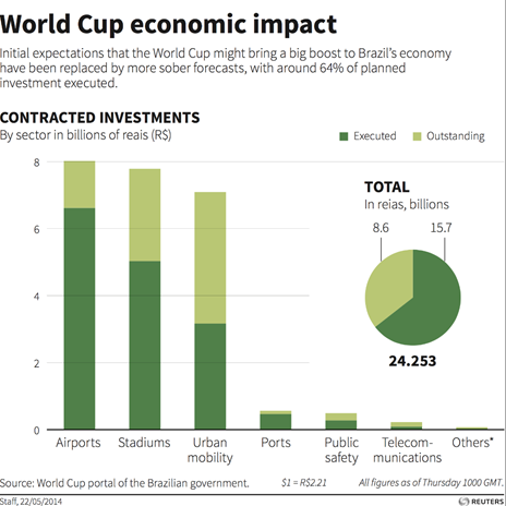
The debate on crypto currencies rages on. The most popular debate hovers around the questions of broader acceptability of cryptocurrencies, whether at some point in time cryptocurrency usage can become so widespread that they start challenging the stature of fiat money? Would central banks bring cryptocurrencies under their regulatory ambit?  Whether cryptocurrency is just another bubble, which will fizzle out as cost of funds creeps up, from level zero? With respect to the underlying technology, which enables cryptocurrency-namely Distributed Ledger Technology (DLT), there is more consensus on the brilliance of the dataset architecture and its potential. Blockchain, which has caught on popular imagination, is a specific dataset architecture within the broad class of architectures classified as DLT. The most popular used case of Blockchain being the cryptocurrency Bitcoin or rather the facilitation of transactions with Bitcoin.

There is a significant amount of anticipation on potential use of DLT other than cryptocurrency. These typically involve using DLT for facilitating high frequency transactions such as payment, manipulating transactions data, post trade settlement and the like. While DLT in its current avatar is close to a decade old however it continues to fall short of expectations in terms of  basic performance parameters such as speed, scalability and operational efficiency. This has limited instances of widespread industrial scale implementations of DLT, despite generating promising results in ‘proof-of-concept’ stage in several cases. Given the current stage of development of the technology, it may be argued, whether such high-frequency fast response processes are the most optimal use of DLT. In this regard, conventional data base technologies on the lines of RDBMS handles way more volumes, more efficiently at higher speed. However, comparing the weakness of DLT with the strength of conventional database architecture may not be fair.

Among the strengths of DLT is its ability to enable peer-to-peer transactions without the need for a centralized monitoring/administrative entity. Of course, conventional data architectures do not support such functionality. So DLT may require used cases which leverage its strength. It has potential to be used for facilitating solutions to far wide ranging economic challenges which previously did not have the required technical infrastructure. One such use case is technologically enabling an International Currency Union where a global reserve currency may be mined by all member nations ie; ‘Mineable’ Global Reserve Currency-MGRC.It may be called a Worldcoin. Of course, it would require huge global political consensus ( or a major foreign currency crisis), to initiate the thinking and debate in that direction.

The argument for the desirability (or undesirability) of a new global reserve currency or a new global monetary order is outside the scope of the current piece. As such, the period from 1971 to 2008, which was characterized by the fiat currency form of US dollar as global reserve currency, had experienced high global growth with relatively lesser number of financial crisis/instability than most periods in history. Only the period from 1945 to 1970, had possibly experienced higher financial stability and more balanced growth than the period 1971 to 2008. However, the 2008 crisis ,and its aftermath, challenged quite a few economic assumptions including the existence and concept of ‘a’ global reserve currency issued by a sovereign i.e.; USA. Global policy response to 2008 crisis ranged from Unconventional Monetary Policy (UMP) to fiscal austerity. The jury is still out on the success of these measures, though strong expectations remain of a global economic recovery. The debate of global reserve currency revived because the trajectory of US economy and strength (or weakness) of USD has taken the world economy on a roller coaster ride. Particularly vulnerable being the emerging markets and developing markets .Such countries face strong challenge to improve the quality of lives of economically weaker sections and such efforts get sidetracked in the event of external financial shocks.

Arguably, regulators and fiscal policy makers have exhausted their box of economic tools with which to fight future financial crisis as well as address structural issues such as global fiscal and trade imbalance. We, given this background, create a case for usage of technology enabled economic tools such as a ‘mineable’ global reserve currency (MGRC), not issued by a sovereign or a group of sovereigns (example Special Drawing Rights-SDR). This MGRC may leverage DLT dataset architecture, while harnessing available enhanced computation power and big data capability to capture ‘live’ data on global trade and financing to facilitate algorithms, which will enable mining of the proposed Global Reserve Currency (GRC). Of course, some bitcoin enthusiasts have been, for some time, propounding that bitcoin itself may be a GRC but it is bit far-fetched unless it has wider public acceptance and explicit backing from governments.

Very Brief History of Global Reserve Currency and Foreign Currency Regime

Prior to World War I, it was the era of “commodity money”. The value of the money was driven by the value of gold, silver or copper contained in the coin. Exchange value of coins issued by different countries was driven by the inherent value of the coin i.e. quantity of the commodity in the coin and the ongoing price of the commodity. As such, the volatility of foreign currency exchange was lesser. In fact, because of the commodity nature of the coins the exchange rate to an extent was delinked from the underlying fundamentals of the economy that issued them.

When in mid-19^th century paper notes started replacing commodity coins more widely, the paper coins retained the essence of commodity money. The paper notes were backed by promise of the issuing government/authority to replace it with gold/silver. The value of the paper note was driven by the amount of gold/silver that was promised by the issuing authority. This often introduced volatility or run on a currency, when the users of the note doubted the government’s ability to replace it with gold/silver and went ahead with demanding the commodity promised in the coin.  In normal times, the exchange rates of such paper notes was driven by the amount of commodity the respective issuers/government promised with volatility getting introduced in the exchange rate in instances where people doubted the ability of the issuer to honor its commitment.

The First World War (WWI) ended commodity money when Great Britain, the issuer of sterling-the global reserve currency of the period, suddenly discontinued specie payment i.e. the bank notes ceased to be exchanged for gold coins. Post WWI financial instability aggravated and an effort was made by Britain in 1925 to return to gold standard, only to finally withdraw it in 1931. And thus Pound Sterling, which was gradually losing its stature as a global reserve currency to US Dollar, started to float.

The next pit stop in this story was the Bretton Woods Conference 1944. The Bretton Woods Conference debated on two proposals for a global monetary and foreign exchange regime. One was proposed by Harry Dexter White of USA and other was by John Maynard Keyes of United Kingdom. Keynes proposed an International Clearing Union (ICU), which would have issued a universal monetary unit of account called Bancor. ICU would be a multilateral body, keeping account/issuing Bancor, and thus no single country would have an overarching influence on its functioning. More details on ICU and related proposals are discussed later. The conference ultimately adopted White’s proposals, which among other things had a Stability Fund, which would have provided for much needed post war reconstruction of Europe. White’s proposal suggested that currencies have a fixed exchange rate against US Dollar which in turn would be convertible to gold. The proposal banked on member countries to issue currency to the extent of its gold ownership so as to maintain its exchange rate with respect to USD. For small deviations or imbalances, International Monetary Fund (IMF) was expected to step-in with support.

 Between 1944 and 1970 there was a period of relatively high financial stability and growth particularly among the signatories of the agreement. USD was formalized as the global reserve currency. However, on August 15, 1971, US unilaterally discontinued the convertibility of USD to gold. With this, the USD became the first fiat money, not backed by gold, to become the global reserve currency. And it continues till date.

Post the Global Financial Crisis of 2008 when the balance sheet of US Federal Reserve expanded due to unconventional monetary policies including quantitative easing, it drove global monetary policy making to unchartered territory. Trade imbalances which was already on the rise pre-2008, surged. Currently, it appears that the health of emerging nations depends on US continuing its high fiscal deficit. The moment there is any plan/discussion in US on correcting its fiscal position or reducing the Fed’s balance sheet, there is often a capital flight of differing intensities in emerging markets. At some point in time, in not so distant future, central bankers and global regulators would need to find a way out of this dilemma. However, it appears that post-Keynesian / Monetarist /Neoclassical economics may not be having potent tools in its toolbox to handle this challenge.

Alternatives to current Global Reserve Currency- from Keynes to Stiglitz

Gessell to Keynes: The idea of a global reserve currency, which is issued by a supra-national entity as opposed to a sovereign in neither new nor recent. Back in 1920, Silvio Gessel, an economic thinker, proposed an institution called IVA-International Valuta Association, which was to issue a global monetary unit called Iva.  The most prominent proposal on alternate monetary system was devised by Keynes and subsequently proposed at the Bretton Woods conference as UK’s official proposal. The basic tenet of Keynes’ proposal was the establishment of an International Clearing Union (ICU) based on an international bank money called Bancor meaning bank gold (in French). Bancor was proposed to be accepted as equivalent of gold for settlement of international balances. The union would not be linked to any one country but would be run as a multilateral agency.

Keynes realized that being the issuer of global reserve currency, as Pound Sterling was prior to 1940, was not an unmixed blessing. It almost always pushed the issuer to have unsustainable level of current account deficits with its ensuing deflationary overhand on the economy. Apparently, the seigniorage that the global reserve currency issuer charged to other countries came with a price.

Countries could hold Bancor as reserves as opposed to holding sterling, dollar or gold as reserves. The immediate benefit being, resources that remain trapped and thus passive as reserve could be released for funding real economic activity. The countries could, depending on their trade position, lend or borrow from the ICU. The union was expected to function as a supranational bank, where the credit of one country may be lent out to a debtor country. While similar financing transactions can be done using bilateral agreement, having a supranational quasi banking union can perform this function more seamlessly for pure economic considerations as opposed to possible political overhang which sometimes are inherent in bilateral financing transactions. The plan proposed a Governing Board to enforce fiscal and monetary discipline among the members.

The plan was intended to have a stabilizing impact on countries with payment or fiscal imbalance. In case of a surplus or deficit of even a quarter-year, the country would have to pay the ICU a charge of 1% per annum. Thus explicitly penalizing members for imbalance. If countries with deficit wants to extend their deficit by more than a quarter then the country needed to seek the Board’s permission. If the deficit exceeds a pre-determined threshold, the country may de-value its currency with respect to Bancor, to the extent of 5%- above which it would again have to seek the Board’s permission. The Board would be responsible for providing guidelines to countries to regain their trade balance.

Certain aspects of the proposal were difficult to implement then as it is now. However, the underlying construct of the plan as well as quite a few operational aspects of the plan continues to remain relevant if one considers a global reserve currency issued by a supra-sovereign institution. In Keynes’ original plan, founding members at initiation stage will set the value of their currency in terms of Bancor/Gold. Subsequent members would have to set the exchange rate in discussion with the board. Significant changes on exchange rate would have been allowed only with permission of the board.  Likewise countries with surplus, which exceeds a pre-determined threshold for a quarter, would have to consider appreciating its domestic currency against Bancor. Alternately they could consider expanding its domestic credit or increasing money wages.

The idea may appear ‘unbelievable’ in this day and age of market driven foreign exchange rate. However, it must be remembered that market driven foreign exchange rate is a phenomenon, which came into being in 1970s after US Dollar was delinked from gold and became a free float. Even today absolute ‘value’ of a currency is not determined, one at best estimates the relative value of a currency against a basket of currencies or estimates likely future exchange rate of a currency with respect to another currency  based on their respective inflation rates. And even in the last four decades no unambiguous framework exists which will tag a currency  as ‘over-valued’ or ‘under-valued’  the way one would describe the value of equity of a company.

Keynes’ proposal included formula for calculating maximum allowed debit balance which was supposed to be the country’s quota. It will be based on the country’s export and import for last three years. Keynes also highlighted other factors to fine-tune the calculations. For 1940s this was computationally intensive but in 2020s with its ability to capture real time trade data and cross border financing data, one may not only implement more involved rules for quota calculation but clearly it is within the domains of technological possibility.

For quite a few years, it appeared that the global trade imbalance would cause a breakdown in international relations and trade; but nothing of that sort happened. However, the world needs options to move out of this current imbalance, considerations for an ICU-like framework may be relevant. In fact in the last couple of decades, particularly post 2008, several economists and thinkers have proposed frameworks which are based on ICU or frameworks which will achieve similar objectives.

Paul Davidson and International Monetary Clearing Unit: Paul Davidson improved on Keynes’ plan in an effort to make it more relevant to the economic and international political realities post 2000; since he did not consider the supranational central bank architecture suggested by Keynes to be either feasible or for that matter necessary.

His solution was for a “closed, double-entry bookkeeping clearing institution to keep the payments ‘score’ among the various trading nations plus some mutually agreed upon rules to create and reflux liquidity while maintaining the purchasing power of international currency”. On the lines of Gesell’s Iva and Keynes’ Bancor , Davidson proposed ‘International Money Clearing Unit’(IMCU) which will be the global reserve currency to be held only by the central banks of the member countries.  ICMU can be transacted only between central banks and International Clearing Union. The private transactions will be cleared between the central banks accounts held with the clearing union. This is analogous to how money from one account-holder in a bank gets transferred to another account-holder in another bank through clearing facilities and involves adjustments against the reserves/deposits of the banks with the central bank.

The exchange rate between ICMU and local currency will be fixed and as per Davidson’s proposal will alter if efficiency wages change. ICMU value in local currency terms will also be driven by domestic inflation rate. This is to control for undue volatility of foreign currency and also reduce speculative attacks on currency. For excessive imbalances a country would have to take steps similar to Keynes’ plan.

Global Greenback Plan: Joseph Stiglitz and Bruce Greenwald proposed a Global Greenback system which was per se not a new global reserve currency but using the ‘Special Drawing Rights’ (SDR), as international reserve. However to the extent SDR is itself a basket of six currencies (latest addition being Chinese renminbi) a lot of the shortcomings identified by Keynes with respect to a global reserve currency being issued by a single sovereign would hold.

Thus, if the world ever goes more a mineable global reserve currency it is likely to have features closer to Keynes’ Bancor or Davidson’s ICMU.

Basics of DLT and Cryptocurrency[1]

DLT is a class of database architecture. A specific type (and of course the most talked about) of DLT is Blockchain. Blockchain caught onto popular imagination because it enables Bitcoin, the most popular cryptocurrency. DLT allows for accessing and updating database from multiple nodes (i.e.; Computers/CPU associated with a user/users) which may be in geographically different locations . The integrity/accuracy of the database is ensured through validation procedures which require consensus of all or some select nodes. As such, the concept of distributed access of a database or simultaneous access across physically different locations is neither new nor unique to DLT. In conventional databases, the storage of data could have been spread across multiple computers and accessed across different nodes. However there was one version/one view/one instance of the dataset at any point in time. The integrity/accuracy of the data depended on centralized data administration capability. Requests for addition to the database or updating existing records would be vetted/validated by data administration before it got reflected in the database. The centralized data administration capability may be called a ‘trusted authority’.

So a payment facility whose IT infrastructure consists of conventional database (which, as of today, is almost all) is likely to operate as follows. When a payment is made the payer’s account is debited and the payee’s account is credited and the system is updated to reflect the updated account status. The trusted authority is responsible for ensuring that the system correctly and promptly captures the transactions and reflects the latest account position. Other authorized, systems can access the central database to find the state of the payer and the payee

The ‘problem’ of course is that the trusted authority has tracked the transaction i.e. the transaction is not anonymous. In DLT there is no trusted authority i.e. no centralized facility to ensure data integrity. In that sense a ‘Distributed’ Ledger is sometimes called a ‘mutually distributed ledger’ to underline the fact that the ownership of data integrity is on the entire set of participating nodes and not just on some centralized data administrator.

 In DLT, the users (node) of the distributed system each have a copy (instance) of the entire database. Once a new transaction event occurs, it has to be updated at each of the instances, which may be accessed by one or more nodes. A transaction is successfully ‘updated’ when each of the nodes has given their consent to the transaction. A transaction event finally gets reflected in the database or rather all instance of the database when all nodes with validation authority have accepted the transaction as valid. As such this process is time-consuming and even when a bona fide transaction event happens, there is only a probabilistic finality of settlement. In many situations, the final settlement can actually take several hours.

Within DLT, the specific workflow, which enables the consensus/validation, differs leading to different type of DLT. As such a validation framework based on simple majority (with each user/node having one vote) would expose the system to attackers who would simply proliferate nodes to game the system. To take care of such possibilities, complex validation protocols were developed.  One framework of validation is ‘Proof of Work’(POW) where the ‘proof’ consists of solving mathematical problems requiring significant computation power, thereby increasing the hurdle of one or a small number of attackers to game the system. Another competing validation framework is a “Proof of Stake”(POS) based consensus . The rights of validations of the nodes depend on their stake in the system. The measurement of stake also has several alternatives in the sense the stake can be measured by the number of token/cryptocurrency the nodes own or number of units of cryptocurrency the node is willing to bet on that transaction.

While thus far we would have got an idea of the distributed nature and technological aspects, one question still remains unexplored. Why is it called a ‘ledger’ as opposed to a database? Ledger usually refers specifically to a functionally of a database where one keeps track of which entity owns how much on a product/value/unit and subsequently how those units are getting spent or further units accumulated. The concept of Ledger is very critical for a non-physical/digital currency, operated in absence of a trusted authority, to prevent double-spending of the same unit.

Efficiency and Choice of Access and Validation: A DLT can be further characterized on two dimensions: i) Accessibility and ii) Validation Right. In terms of accessibility the options are broadly two namely Public, where any user is allowed to read/view the ledger and Private, where access is limited to users with explicit access rights. Validation rights refer to who can validate or make changes in ledger. Here the two options are, permissioned where only a subset of all users who are specifically identified can validate/modify the ledger. The other option being Permission-less where all users are allowed to add/alter/validate the ledger

 The way popular cryptocurrency transactions are facilitated by Blockchain typically follows public, permission-fewer frameworks. Needless to say this process takes a lot of time and computation power. From a user perspective when bank money is transferred, it takes seconds or few minutes to confirm the transaction to the parties. In DLT the transaction confirmation sometimes takes hours. Financial services are used to electronic payment networks which process upwards of 25,000 transactions per second. In comparison large block chain network processes less than 10 transactions per second.

However, for the purpose of a mineable Global Reserve Currency it may be envisioned that it will be a Private and Permissioned protocol, so speed of the transactions may not be an issue. As such an idea such as MGRC may take at least a couple of decades to implement unless of course there is a major crisis pushing global consensus on such a move. While the technology around DLT and Blockchain is close to a decade old and certain commentators still consider the scalability and power usage as a bit underwhelming, it may be hoped that these issues will be resolved with time.

Economics of Cryptocurrency: Currency is a subset of a broader economic concept of money. Currency is the ‘token’ which facilitates movement of money, shifting its purchasing power from the current holder to its future holder. Currency facilitates the exchange feature of money i.e. payment. Currency, driven by technology has evolved into several forms; from good old cash/coins, to electronic money and more recently cryptocurrency. Currencies are typified by key features namely physical existence, issuer, ultimate liability, universal accessibility and peer-to-peer exchangeability. Cash ticks most boxes i.e. exists physically, issued by central banks with ultimate liability being that of the government, universally accessible within the jurisdiction and can be anonymously ,at zero cost, used in peer-to-peer exchange. Electronic money represents electronic payments facilitated by banks, payment networks differ from cash as they do not have  physical existence and finally, peer-to-peer exchange are tractable by authorities and hence anonymous like cash.

A Cryptocurrency addresses the need to enable peer-to-peer anonymous transaction on the lines of cash. However cryptocurrency provides this anonymity in online/electronic transactions which credit card/debit card/internet banking based payments cannot. This explains the ‘crypto’ aspect of the cryptocurrency.

Suggested Framework of a Mineable Global Reserve Currency (MGRC)

The first version of Basel norms (Basel I) had, in comparison to the current banking regulations, relatively simpler framework for capital requirement. Still it took 14 years of negotiation (started in 1974, as Basel Committee on Banking Supervision) by central banks of the group of 10 countries (7 European, USA, Canada and Japan). These countries had largely similar econo-political orientation. If typical WTO negotiations are anything to go by, a coordinated, globally synchronized effort to create a new monetary framework would easily take a couple of decades. Previous instances of synchronized effort to shift to a new monetary regime took earth-shattering events like a couple of World Wars. So technological feasibility of a MGRC is the least of the roadblocks. However, the frequency and intensity of the debate around the MGRC can increase since it is an issue of global political intent and not of technical ability.

The proposed framework is dependent on the current state of technological sophistication of the DLT. It is not expecting any significant improvement on the same. Since Keynes had designed the first detailed framework, the proposed framework, in his memory, may be called International Currency Union-ICU and the MGRC may be named as WorldCoin

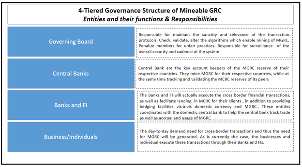
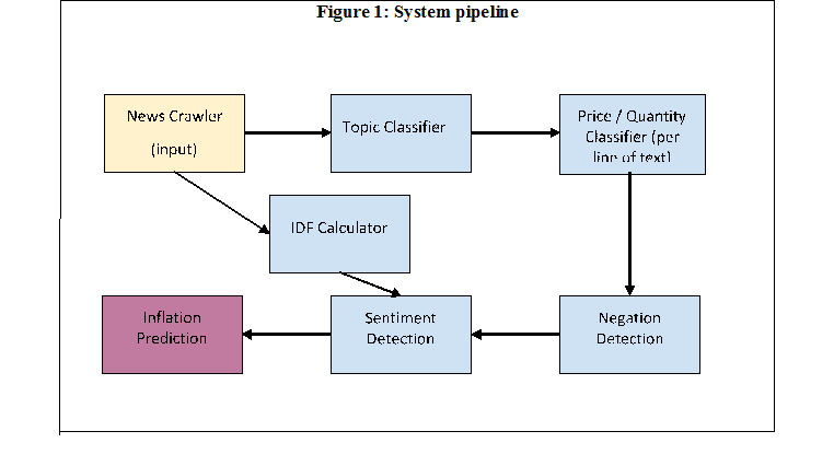
Governance Structure of ICU: The ICU may consider a four-tiered administrative structure. The overall enablement and infrastructure support may be under the Governing Board. The Board would have representatives from all members; however a sub-group selected by rotation may make the core decisions on an ongoing basis. The stewardship of the core decision-making group may be rotated on a periodic basis among member countries. The Board would interact directly with the respective Central Banks of the member nations.

The central banks would be responsible for maintaining the accounting and cadence framework, which will justify the conversion rate of local currency with respect to MGRC. Most importantly, the central banks are the entities who will be responsible for actually ‘mining’ the MGRC based on the trade and macro parameters. Central banks are best placed to do so since in most countries they are directly responsible for determining their domestic money supply/credit supply, which ultimately influences inflation and growth.

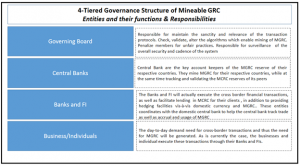
Banks and Financial Institutions regulated by their respective central banks will facilitate the transactions in MGRC. Specifically, these regulated financial institutions will be responsible for executing cross border financial transactions where the underlying is MGRC. Foreign currency transactions being facilitated by domestic banks is also the case today, under the proposed scheme of things the foreign currency will be replaced by MGRC.

Operational aspects of accruing and accounting MGRC: The central banks would be responsible for keeping track of the MGRC account with respect to its country. The MGRC reserves of a country will keep on fluctuating constantly, for reasons pertaining to business and economy, which will largely be same set of reasons which cause fluctuation in value of current reserve holdings. Currently, typical reserves of most countries constitute some combination of USD, SDR or currencies in SDR and Gold. An incremental source of accruing MGRC will be ‘mining’ the MGRC based on positive trade/cross country financial trade data.

At the lowest level (Level 1), demand (outflow) and supply (inflow) for MGRC will be attributable to trade of Goods/services between businesses/individuals domiciled in different countries. A net positive export (by value) will cause the country to earn(net) MGRC and increase its MGRC holding while the opposite impact will happen if the country is a net importer. The trade (payment aspects, specifically) will be facilitated by banks and financial institutions, as is the case today. Under a proposed MGRC framework, the business will earn or spend in terms of MGRC (as opposed to, say, USD/EURO/JPY today) and they may be allowed to hold MGRC accounts with the bank. For calculation of profits or financial reporting purposes, the conversion rate of MGRC with respect to the local currency needs to be used. For that matter if a business/individual wants to convert its/his MGRC holding into local currency, and vice-versa, it can be execute based on the conversion rate.

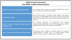
The Level 2, consists of financial institutions which will facilitate international trade related payments. This intermediation function will not incrementally alter the MGRC reserve of the country over and above what is contributed by the underlying business and trade. However, to the extent these financial entities start providing MGRC related hedging tools (against change in conversion rate of local currency vis-à-vis) and loans denominated in MGRC, they will affect the MGRC reserve of the country. For the MGRC loans extended to businesses/individual by their respective domestic banks, the domestic bank may disburse the MGRC loan from various sources such as its own MGRC account, it may borrow from the central bank, or it may borrow MGRC from another domestic and international bank for onward lending. This is also the layer, which will absorb the capital inflows/outflows. Thus if FDI flows into a country, denominated in MGRC, this is the layer which will facilitate the monetary elements of the transactions

Level 3 is the layer where only the central banks of respective countries operate. Central banks constitute the only entities which are allowed to mine the MGRC and add to the country’s MGRC. The mining algorithms may be determined by macro factors’ such as inflation and fiscal deficit. Recall separate capital account deficit or trade deficit need not be considered in the mining algorithm as their impact on MGRC reserve will be deterministically captured in Level 1/Level 2 .

Level 4 is the topmost layer, which can add/reduce the MGRC reserves. This is bilateral borrowing between nations. For example, nations whose demand of MGRC is rising much faster than their ability to earn the same and who have weak economic parameters which prevent them from mining new MGRC, the MGRC will appreciate sharply against their domestic currencies. In such cases the country in crisis may borrow MGRC from another country with comfortable MGRC reserves. Such borrowings would increase the MGRC reserve of the borrower and reduce MGRC reserve of the lender.

Operational Details of Cross-Border MGRC Transactions: If a business in a country wants to make a payment to a foreign company/individual through MGRC, the set of transactions will be analogous to the transfer of money from one bank account to another bank across the border. In the current framework, the DLT will enable live tracking of the MGRC account at not only the business or bank level but it will get updated at the Central Bank level, so that ultimately the Governing Body of the ICU knows the MGRC holdings at country level. Additionally the countries are aware of each other’s MGRC level that will build higher level of trust and would address issues of currency manipulation.

Conclusion: The option to have a Global Reserve Currency, which is not issued by any one sovereign, needs to be actively discussed. In the scheme of things, the entire world paying seigniorage to a single country is possibly the least of the issues. As Keynes has identified the problem with a single sovereign issuer of reserve currency, which used to be the case with UK and Pound Sterling prior to 1930, the system can operate ‘well’ only when the issuer country runs a large deficit. This imbalance attributable to continuously running deficits, even in absence of a major economic shock, will push the issuer towards a deflationary economic environment. In the event of a major crisis such as in 2008, US had to resort to unconventional monetary policy in a bid to prevent a repeat of the 1930s recession. Not just US, issuers of major currencies such as Pound, Yen, Euro have adopted some version of unconventional monetary policy. These countries will gradually try to move towards normal monetary environment (i.e., non-zero interest rate, no excess liquidity via quantitative easing)  This ‘normalization’ of monetary policy may reduce funding liquidity, and also limit credit/money supply. The steps and the outcome are largely outside the domain of usual hypothesis/deductive reasons applicable to prevalent macro thinking. It may be fair to assume that each of these countries will try to safeguard their own national economic interest before anything else.

If the unwinding of the existing near zero interest regime and normalization of a liquidity deluge environment is relatively painless for other countries, then possibly there will be not much trigger for discussion of a country neutral GRC. However, if there are widespread market disruptions or economic shocks, that may provide an opportunity to discuss GRC, which is independent of the fortunes of an issuer country. In fact, a country-neutral GRC may prevent foreign currency contagion in emerging nations. It would of course mean a shift towards a new monetary regime globally and may potentially challenge or disrupt the functioning of FX currency markets particularly its most important constituency- FX traders.

The DLT comes closest to providing the ideal technological infrastructure for MGRC. To enable transparent, real-time tracking of reserves as well as ‘mine’ the reserve currency without day-to-day centralized intervention by any authority, a Blockchain like data architecture may be useful. Apart from building trust in the system it will reduce dependency on the economic fortunes of any one country. To the extent that the Central Banks themselves will be the direct users of this peer-to-peer system, the information is unlikely to be used by manipulative elements in currency markets.

As far as using the concept and framework of MGRC is concerned, the framework can be tweaked to create a two-tiered monetary structure say for instance in Eurozone. Where the Euro can become a currency of exchange in trade in Eurozone (as of course is the case currently) but each country have their own currency mapped to a ‘Mineable’ Euro. In a relatively smaller scale, the same framework can be used by multilateral trade bodies to keep track of accounts/as well as payments based on mineable currency as opposed to using global reserve currency or the currency of the largest trading member in that trade bloc. The MGRC may possibly, if and when implemented, turn out to be the most important use case of DLT.

Reference

Morten Bech & Rodney Garratt; Central Bank Cryptocurrency; BIS Quarterly Review, September 2017

David Andolfatto, Bitcoin and Beyond: The possibilities and pitfalls of virtual currencies, Federal Reserve Bank of St.Louis, March 2014

Joseph Bonneau, How long does it take for Bitcoin transaction to be confirmed, Coin Centre, November 2015

Gareth W. Peters et al; Trends in Cryptocurrencies and Blockchain technologies:a monetary theory and regulatory  perspective, The Journal of Financial Perspectives Winter 2015

M.Raskin and D.Yermack; Digital currencies, decentralized Ledgers and the future of central banking; NBER Working Paper, May 2016

Josh Ryan-Collins,Tony Greenham,Richard Werner,Andrew Jackson; Where Does Money Come From?

John Keynes; A Treatise on Money

[1] Readers, aware of the basics of DLT and Cryptocurrencies, may skip this section without loss of continuity.

How do we know about the general sentiment in the economy? Is it bullish or bearish? This question seems to haunt academicians and policy makers alike. The best way to gauge it is perhaps approaching the public. The general philosophy is best captured in the burden of Kishore Kumar’s song of Rajesh Khanna starrer movie Roti (1974) that goes, “Yeh jo Public hai – sab jaanti hai“. The question is: where does one meet the public and how does one listen? Does the public whisper or talk loudly? More importantly, does one get a unified message from such public talk or does all information get drowned in cacophony? This paper makes a preliminary attempt to gauge public opinion in newspaper reports. Within this general philosophy, our attempt in this paper is, of course, more modest. We look into one particular economic variable, viz., inflation.

Needless to say, Inflationary expectations tend to play a crucial role in macroeconomic and financial decision / policy making. In particular, it is of paramount importance when monetary policy is conducted within an inflation targeting framework or when the financial market player is thinking of her return from the bond / forex markets. But a perennial question in this context is: how to measure inflationary expectations? Three broad strands are identified in the literature. First, model based forecasts (univariate or multivariate variety) are often taken recourse to. Second, inflationary expectations are also derived from class / group-specific inflationary expectations surveys routinely conducted by central banks / financial data providers. Third, inflationary expectations / perceptions are also inferred from the market yields of inflation-indexed bonds.

While each of these methods is useful, each has its limitations as well. In this paper we propose and adopt a novel method of inferring inflationary expectations using a machine learning algorithm by sourcing economic news from the leading financial dailies of India. In particular, we argue that Economics / Finance can leverage advances in artificial intelligence (AI), natural language processing (NLP) and big data processing to gain valuable insights into the potential fluctuations of key macro indicators and attempt to predict the direction (upward versus downward) of monthly consumer price inflation.

The remainder of this article is organized as follows. While section 2 discusses the motivation of this approach, the methodology is delved in section 3. Section 4 presents the results and section 5 concludes.

2. Motivation and Received Literature

The motivation of this approach can be traced in two distinct strands of literature. First, among the monetary economists there is a large literature of what has come to be known as the “narrative approach to monetary policy”. While the origin of this approach can perhaps be traced to Friedman & Schwartz (1972)’s Monetary History of United States, Boschen and Mills (1995) derived an index of monetary policy tightness and studied the relation between narrative‐based indicators of monetary policy and money market indicators of monetary policy. They found, “Changes in monetary policy, as measured by the narrative‐based policy indices, are associated with persistent changes in the levels of M2 and the monetary base”. More recently, Romer and Romer (2004) derived a measure of monetary policy shocks for the US. Instead of taking any particular policy as an indicator of monetary policy shock, Romer and Romer (2004) derived a series on intended funds rate changes around meetings of the Federal Open Market Committee (FOMC) for the period 1969–1996 by combining the “information on the Federal Reserve’s expected funds rate derived from the Weekly Report of the Manager of Open Market Operations with detailed readings of the Federal Reserve’s narrative accounts of each FOMC meeting”. But all these papers involve some degree of subjectivity of reading the policy narratives. Hence a key question remains: how does one get rid of this subjectivity? It is here that more contemporary tools of machine learning, nature language and big data processing become helpful.

This second strand of literature comes from machine learning. To get a perspective of its emergence, it is important to note that there has been a healthy scepticism and conscious efforts on the part of the academics to avoid forecasting economic / financial variables. Smith (2018) in a recent article attacked the profession and went on to say:

“Academic economists will give varying explanations for why they don’t pay much attention to forecasting, but the core reason is that it’s very, very hard to do. Unlike weather, where Doppler radar and other technology gathers fine-grained details on air currents, humidity and temperature, macroeconomics is traditionally limited to a few noisy variables …. collected only at low frequencies and whose very definitions rely on a number of questionable assumptions. And unlike weather, where models are underpinned by laws of physics good enough to land astronauts on the moon, macroeconomics has only a patchy, poor understanding of individual human behavior. Even the most modern macro models, supposedly based on the actions of individual actors, typically forecast the economy no better than ultra-simple models with only one equation ….whatever the reason, the field of macroeconomic forecasting is now exclusively the domain of central bankers, government workers and private-sector economists and consultants. But academics should try to get back in the game, because a powerful new tool is available that might be a game-changer. That tool is machine learning” (emphasis added).

But what is machine learning? Loosely speaking, “Machine learning refers to a collection of algorithmic methods that focus on predicting things as accurately as possible instead of modelling them precisely” (Smith, 2018). With rapid advances in storing and analysing large amounts of unstructured data, there is increasing awareness that these data could be a rich source of useful information for assessing economic trends. Various attempts have emanated in forecasting macroeconomic and financial variables. Illustratively, Nyman and others (2016) used the Thomson‐Reuters News archive (consisting of over 17 million English news articles) to assess macroeconomic trends in the UK. More recently, using machine learning techniques Shapiro & others (2018) developed new time series measures of economic sentiment based on computational text analysis of economic and financial newspaper articles from January 1980 to April 2015. There is now a burgeoning literature on this issue, thanks to the Rational Expectations thinking that policy making needs to have some sense of the future sentiment / expectations. However, the policy maker needs to take care of the popular adage of Goodhart’s law whereby “when a measure becomes the target, it can no longer be used as the measure”, so that forecasts fail when used for policy prescription and when used as targets naively.

Detection of sentiment from the newspapers seems to be less prone to this syndrome. Much of this literature asks the machine to find out the recurrence of some key words with appropriate identifiers in the newspaper articles so that the detection does not get corrupted by any subjective bias. Our paper ties to decipher the inflationary sentiment from the newspaper articles.

3. Methodology

Literature on sentiment analysis shows that mere frequency of information arrival (news articles) may not explain change in an economic variable. What drives economic agents is the sentiments (i.e., quality) of information. Extracting sentiment from newspaper reports is one of the major contributions of our paper.

We develop a system over python and several accompanying libraries to access large chunks of newspaper data, parse and process the news content, and make a well founded estimate of the direction of inflation (CPI) in the near (next) month using sentiments generated from news content for the current month.

Input: To forecast inflation for a month (released in the middle of the month), we take as input news from 20th of previous month to 10th of current month. We can take as many newspapers as we like. For instance, for inflation of April 2015 (released an Apr 15), we use news from March 20th 2015 to April 10th 2015. Note that CPI numbers are released in the middle of a month (12th to 18th).

Output: For each month, we consume all the input news content and after processing, produce a single number which denotes the sentiment towards inflation for that month.

Component: Our system consists of the following components arranged in a pipeline.

Figure 1: System pipeline

Our search is limited to news from two business dailies (Economic Times and Business Line). We crawl the news from the “factiva” database online using a python tool. This is our input to the rest of the system.^[1] Let us now turn to each of the components of Figure 1.

Topic Classifier

This module takes as input a news article and classifies it into one of the sub baskets used to calculate the overall CPI. The sub baskets are fuel, food, cloth, housing, intoxicants (alcohol and various tobacco consumables) and miscellaneous.^[2] The classifier can classify an article into one of these multiple baskets. We manually labelled about 4000 articles for two random months (Nov-Dec 2015 and 2016) to serve as our training set. It is interesting to note that the training dataset included the period of demonetisation.

Price/Quantity Classifier (Per line of text)

This module takes as input a line of text from an article and flags it as talking of price of the commodity, quantity of the commodity, of both, or of neither. Each line is classified into one of four categories – talking of neither price or production, of only price or only production, or both. The idea is that inflation expectation is triggered by knowledge of either demand pull inflation (higher prices due to higher demand) or cost push inflation (higher prices due to lower supply).

For instance, “Oil prices unlikely to rise” would be classified as talking of only price, “OPEC cuts output on breakdown of talks” would be classified as talking of only production, “While prices seem to be rising, production is not falling commensurately, leading to inventory accumulation” would be classified as talking of both price and production, while “New policies on the horizon” would be classified as talking of neither price nor production.

Negation Detection (Per line of text)

This module takes as input a line of news text and checks whether parts of the line are negated using negation words as “not”, “unlikely”, “improbable” etc. The way it does this is as follows. For example, consider the line: “Oil prices not likely to rise”. The negation detector returns as output “Oil prices <negated scope> not likely to rise <\negated scope>”. The additional markers inform us of the part of the sentence whose adjectives (in this case rise) are negated in meaning. This is utilised downstream in sentiment detection (see example in later section on sentiment detection).

IDF (Inverse Document Frequency) Calculator

TF (Term Frequency) of a word is defined as the number of times a word is seen in an article (document). IDF of a word is defined as a measure of the salience (or contribution to new information) of a word, based on how likely the word is to appear as a prior. If we merely use Term Frequency, we would not account for the fact that words which have a high prior of occurring will bias our estimate. For instance, determiners like a, the, will have naturally high TF, and they need to be downweighted.

This module looks at sentiment words (generally adjectives) which we use downstream to infer sentiment from news articles, and calculates their IDF (Inverse Document Frequency) over our news articles dataset. Hence, for a word which appears in every document, IDF is zero, whereas it is most for a term which occurs in only one document.

Our IDF is calculated based on the news articles for the first six months of our dataset (months of July-December 2015). This should have broad enough coverage to give us a principled and correct estimate of IDF.

Sentiment Detection

This module takes as input an article, and rates each line of text in the article with a number which describes whether the line indicates a rise or a fall in inflation. For this, it uses the information inferred upstream – whether the line talks about price/production, its negated scopes, and the relative strengths of sentiment adjectives. Sentiment adjectives which appear closer to the mentions of price/production are weighted more.

Illustratively, consider the sentence “Oil prices not likely to rise”. As explained earlier, this sentence is classified as talking of price (due to the word “prices”). Consider the IDF of rise to be 2.0. Consider the dampening factor for interword separation between the adjective (rise)and subject (prices)to be 0.8. We exponentiate the dampening factor to the number of words in between, which is 3 in this instance(not likely to). Therefore, our sentiment score is (0.8^3)*2=1.024. However, the sentence adjectives are negated as determined by the output of the Negation Detection module (“Oil prices <negated scope> not likely to rise <\negated scope>”). Therefore, the value for rise is negated to -2.0, and we end up with a sentiment score of -1.024

After scoring each line, the article sentiment score is simply a weighted sum of the scores for the individual lines. It strongly attributes more weight to the headline and line towards the beginning of the article. This method provides an unscaled number (which takes all real values, but is likely in the range (-10, 10) which determines the strength (and direction) of sentiment of each line in the article. We dampen this unscaled number to a number between (0, 1) (exclusive), using a dampening function function. The higher the number, the more it indicates a positive sentiment towards a rise in inflation.

Inflation Prediction

We follow a short-term prediction approach with monthly updation of parameters. We use individual sentiment values for each article in a month, and aggregates them into a single predicted inflation number for the next month.

We learn a multivariate regression model over our training months, which is as follows:

I (t) = k + aS_food (t – 1) + bS_fuel (t – 1) + cS_cloth (t – 1) + dS_misc (t – 1) + eS_general (t – 1) + fI_dm

  is an indicator variable which is 0 for all months before demonetization and 1 afterwards. This is to inform the model that an external event, which affects public sentiment strongly, has occurred. We note that the introduction of this variable results into a significant improvement in our prediction model. We may introduce such variables for other similar external shocks to the economy, which strongly affect inflation.  is Inflation at time t (month t), and is sentiment for basket ‘x’.

We predict inflation for month i, using the sentiments and inflation figures of month i – 1. Similarly, for month i + 1, we use the actual inflation number for month i, so that our model is improved.

Input Size

Per newspaper, there are about 50 articles per day. That adds up to 1500 articles per month per newspaper. We currently work with two newspapers (Economic Times and Business Line), therefore we have around 3000 articles per month (Table 1).

Each sub basket component of CPI has about 5 – 400 articles per month. The general category is not a CPI component, but we measure sentiment as belonging to this category if an article directly addresses inflation (and does not talk of any of the subcomponents of the CPI basket). This serves as a useful signal to measure sentiment towards overall inflation.

As a rough estimate, misc contains the most number of articles per month at 350 – 400 on average, and the other baskets contain 50 – 250 articles per month on average. There are very few articles (about 7 on average) per month addressing the general category.

4. Performance Metrics and Results

It takes about 60 – 120 seconds of real time on a commodity PC to process an entire month’s news and output the sentiment score for the month. The configuration used is an i5  2.30 GHz processor, with 2 cores and 2 threads per core (although at present we do not use multithreading). Our system is built in python and these measurements were made on Linux. We should note that this is unoptimized code, so within python itself, optimizing should lead to faster performance. Further, using a lower level language and libraries should lead to even faster performance. There is great scope for parallelization in our system, since each article is processed independently of the other. Leveraging this could lead to orders of magnitudes improvements too.

We calculated monthly sentiment for each of the CPI baskets and performed a univariate regression of basket sentiment on basket inflation. We found high univariate correlation for the food, fuel, cloth and misc baskets, as well as high correlation between sentiment for the general category and overall inflation. The results are given in Table 2.

Further, the multiple regression leads to a high significance for fuel, food as well as general sentiments. Table 3 reports the regression results.

I (t) = k + aS_food (t – 1) + bS_fuel (t – 1) + cS_cloth (t – 1) + dS_misc (t – 1) + eS_general (t – 1) + fI_dm

Prediction Results

How is the predictive performance of the model we have developed? The figure below charts a scatter plot of true inflation versus predicted inflation using our model. We achieve a correlation score of 0.59.

Figure 2: Inflation (True versus Predicted)

5. Concluding Observations

Measuring inflation expectation is a key component of economic and financial policy making. We use text mining to predict inflation expectations. This experiment of investigating whether inflation perception can be measured using newspaper text essentially consists of two sub experiments. The first is to check how well an automated system, when invoked on a single newspaper article, can infer its general sentiment about inflation. This is to say that if an expert (economist) were to read the same article and conclude that this article says price is going to rise, the system should be able to provide the same result. The second is to check whether given such sentiments about each article, does the aggregated sentiment from the monthly news remain significant and relevant to predict actual inflation numbers.

The first of these subtasks, we must say, has achieved high accuracy. When we evaluated the sentiment inferred by the system on individual articles by hand, the system performed accurately almost all the time, and even corrected the human labeller on some occasions! To this extent we believe that the underlying Natural Language Processing used to generate such sentiment may not benefit much from improvements, as our “simple” model appears to do well. The most significant way to improve this now could be to target a finer level of granularity in terms of inferring article sentiment. That is to say, the challenge is to build a system which not only tells us whether price is going to rise or fall, but also by how much. Note that this task is indeed hard for even an expert to complete.

The second of these subtasks however, may see various improvements. For one, we have yet only observed (largely) direction of sentiment of an article. However, if the article talks about something relatively unimportant, we may wish to discount its contribution to overall sentiment. This may be based on the commodity it is talking about, its source, the tense of the text, and the timing of the article (within our prediction horizon which is monthly), none of which we have yet included in our model. Future work in this direction may aim to incorporate such factors.

One of the principled limitations of our approach is that in a developing country like India (versus say, the United States), financial news often does not percolate (fast enough) to the rural population. Hence, using only financial news sentiment to measure perception towards inflation may not be good enough. To this end, we performed our predictions (as above) on urban inflation instead of overall inflation, and saw a slight improvement in results.

Of course, one of the crude ways to improve our system further would be to use more newspapers, and to use more labelled data. We could also include other measures of public sentiment for inflation, in the form of well-read blogs, news published by the central bank in press releases, and even social media data such as twitter posts.

This is a novel, if not the first attempt, to quantify public sentiment towards inflation by inferring it from newspaper text for India. Besides, it compares well with the IESH (Inflation Expectation Survey of Households) conducted by the RBI in order to measure inflation perception as IESH achieves a correlation coefficient of 0.50 in predicting the actual inflation figure, whereas we obtain 0.59 with our method. We hope that such approaches to predicting macroeconomic variables are investigated further by the research community, and fruitful results applied in public policy making.

References

Boschen J. and S. Mills (1995): “The relation between narrative and money market indicators of monetary policy”, Economic inquiry, January, pp 24-44.

Friedman, Milton and Anna J Schwartz (1972): A Monetary History of United States, 1867 – 1960, Princeton: Princeton University Press.

Nyman, Rickard , David Gregory, Sujit Kapadia, Paul Ormerod, David Tuckett & Robert Smith (2016): “News and narratives in financial systems: Exploiting big data for systemic risk assessment”, Bank of England Working Paper No. 704.

Romer, Christina D. And David H. Romer (2004): “A New Measure of Monetary Shocks: Derivation and Implications”, American Economic Review, September, 94(4): 1054 – 1083.

Shapiro, Adam Hale, Moritz Sudhof, and Daniel Wilson (2018): “Measuring News Sentiment”. Federal Reserve Bank of San Francisco Working Paper, available at https://doi.org/10.24148/wp2017-01

Smith, Noah (2018): “Want a Recession Forecast: Ask a Machine”, Bloomberg, May 13, 2018, available at https://www.bloomberg.com/view/articles/2018-05-11/want-a-recession-forecast-ask-a-machine-instead-of-an-economist

^[1] We are in the process of extending it to use news from “Business Standard” and “Financial Express”.

^[2] The relevant weights for each of these groups are 45.86%, 2.38%, 6.53%, 10.07%, 6.84%, and 28.32%, receptively.

This issue deals with valuation of pre-revenue companies. We define a pre-revenue company as one, which has already completed prototype and obtained customer validation. The company may or may not have some revenue. The fact that the company has produced prototypes/proof of concept implies that ideation stage is over and customer validation further demonstrates that the product/service will have commercial acceptability. Investment at such an early stage is highly risky. Therefore, angel investors at this stage will only seek scalable investments- companies that can grow revenues very fast within five to eight years. The potential to scale up operations at a greater pace in early years depends solely on the quality of founders and the leadership team.

There are two popular methods to evaluate a pre-revenue company: the scorecard method and the venture capital method.

The Scorecard Method 

This is a qualitative framework to evaluate fundability of a start-up that has no or a few small-ticket customers. At this stage of a start-up, it is impossible or futile to judge its viability on the basis of financial projections. The scorecard method, therefore, relies on broad factors that are essential for the success of a business plan. This method tries to raise relevant questions to evaluate size, scalability and sustainability of a business. The questions posed should be as objective as possible so that a score can be assigned to each question. Decision to fund a start-up at this stage depends on the overall score obtained. A prospective investor may have a threshold score to fund any early stage start-up. Start-ups securing a higher score would have greater probability of funding.

An early-stage investor evaluates a pre-revenue company on the basis of the following criteria: (a) strength of the management team; (b) size of the market opportunity; (c) level of competition; (d) implementation plan; and (e) funding required.  Each criterion will have weights ranging from highest (25-30%) for the management team and lowest (5-10%) for funding requirements. An investor will design several questions for each factor (criterion) and assign marks/scores. For example, founder’s experience and willingness to step aside for a new CEO, if necessary, could be important questions to evaluate strength of the management team.  Often an inventor may be the bottleneck for scaling up of operations. The innovator may have great knowledge of the product but very little idea about how to run an organisation or even how to take the product to the market. In such a situation, any prospective investor may insist that the funding may be conditional on the founder’s willingness to handle over the operational responsibility to a professional CEO. If the founder is unwilling, that may turn out to be a deal killer. On the other hand, if the founder voluntarily makes such a transition a key part of the business plan, the investor will be impressed and put a higher score. Similarly, size of the specific market and potential revenue in five years could be relevant questions for understanding the size of the market opportunity. If the market opportunity is small, no investor may be interested in the business even if it has a great team and product.

Table 1: Illustrative Scorecard

If the product or service is patentable and the founders have obtained necessary patent, it increases the entry barrier. A higher entry barrier would reduce competition in early years of the venture and such a start-up should be able to attract funding. Implementation plan of the business should be unambiguous and actionable. An important factor at this stage is to identify sales channel that can support the projected growth. If product facilities are required, the founder should be able to clearly state whether production will be outsourced and vendors are identified. If production were to be done in-house, a related question would be whether land is available and how long will it take to build the production facilities. In the early stage, investors prefer that manufacturing is outsourced so that funding requirement is moderate.  Finally, if the ask for fund is high at pre-revenue stage, chances of getting positive response from prospective investors are remote. Funding up to $1 million may be available at this stage if the overall score is high. If the requirements for fund are higher, it is quite difficult for a start-up with no revenue to generate enough interest among early-stage funders.

The Venture Capital Method

The venture capital (VC) method is an optimistic method, which only considers successful scenario of a business. It is used at a stage where the start-up has clocked some revenue to demonstrate that its product/service has market acceptability. The VC method assumes that the start-up, it is considering for funding, will be successful.  It asks the entrepreneur to predict the revenue of the business at the end of five or seven years. It, therefore, assumes that the business will survive till such time and would generate the target turnover. Of course, the entrepreneur will have to justify the projected revenue and the investor would ensure that the number is not too optimistic. Typically, at pre-revenue stage, entrepreneurs show non-linear growth in revenue in early years on the assumption that necessary funding will be available and the management team would have the capacity to manage such significant growth rates.

Once the projected revenue is estimated, the VC method requires two more variables to arrive at the post-money valuation- the revenue multiple and an appropriate discount rate. Post-money value refers to the value of the firm assuming the enterprise receives the required funding. If one deducts the investment from post-money value, one gets pre-money value.  The value of a firm in VC method with an exit after N years is given by :

Enterprise Value= [Projected Revenue at the end of year N * P/S Multiple]/(1+IRR)^N

The revenue multiple should be chosen in such a way that a fair value can be obtained. Here, the funder has to decide about an appropriate multiple. This would involve identifying comparable firms and their revenue multiple at present level. For example, if the start-up is an online food delivery service company like Swiggy, and Zomato, one needs to obtain the revenue multiple at which these start-ups have raised money recently. Swiggy’s revenue in FY 2017 was reported at Rs. 133 crore versus Rs. 20 crore in FY 2016- registering a phenomenal growth in top line.  Swiggy had raised $80 million in May 2017 at a total valuation of $400 for the company.  If one uses the FY2017 turnover of Swiggy, this valuation implies a staggering Price-to-sales (P/S) multiple of 195! Swiggy has further raised $100 million almost a year later (February 2018) at a valuation of $600 million. So, the revenue multiple has gone up in anticipation of even a higher revenue growth in FY 2018. It is interesting to note that even when revenue grew by six times for Swiggy in FY 2017, losses too grew by 50% to Rs. 205 crore. It is clear that investors at early stage of a start-up fund growth and are not bothered about profitability. Swiggy’s competitor, Zomato, raised $200 million at the same time (February 2018) when it reported overall revenue for FY 2017 of Rs. 333 crores  (81% more than last year) and revenue from online ordering of Rs. 58 crore (eight-folds higher than previous year). Zomato raised the latest round at a valuation of $1.1 billion resulting in a sales multiple of 21. Later Morgan Stanley[1] raised the valuation of Zomato to a whopping $2.5 billion on the basis of expected revenue of Zomato of $65 million in FY 2018, implying a revenue multiple of 38. Another related start-up, Grofers (online grocery), has recently raised $61.3 million at an enterprise value of $300 million[2] and reported an annual turnover of Rs. 1000 crore ($154 million). This implies a modest P/S of 2. Possible reason for such a low multiple could be the fact that Grofers was struggling for the past two years with its business model and witnessed more than 30% drop in its valuation. Two important lessons from the story of these three start-ups are: (a) there is a great deal of optimism with these start-ups in view of such high P/S multiples; and (b) the variation of the multiples is huge. Such wide variations make it difficult for an investor to use these numbers as benchmarks to value any pre-revenue start-up in the same sector.  So, what should be an appropriate P/S multiple for a pre-revenue start-up given the two recent success stories of Swiggy and Zomato?  Will the pre-revenue company be able to generate levels of revenue growth shown by these two start-ups in five years?  If the answer is affirmative, one can use a conservative P/S multiple, which is about 30 (closer to Zomato). One may note that Zomato has achieved the present multiple after ten years of struggle.  If the answer is in the negative, one may use P/S multiple of listed comparable firms, if available.

The preferred discount rate (also known as internal rate of return) of the investor should take into account the following four factors: (a) time value of money (as the exit from early stage investment is prolonged, it is essential that one uses yield of long-term government bond for this purpose); (b) premium for market risk (as the valuation is sensitive to market factors); (c) premium for considering only successful scenario (since the VC method does not consider probability weighted scenarios); and (d) premium for possible dilution in equity (there could be possibility of subsequent rounds of funding before the exit of early-stage investor). Therefore, the preferred discount rate would be much higher than the traditional cost of capital measure that uses only the first two factors.  It is not easy to estimate the last two factors. One way to measure the premium for successful scenario is to collect information on start-ups that are successful in raising multiple rounds of funding in first 7-10 years. The difference in the valuation of these start-ups between the first round and the latest round of funding can be explained by increase in earnings and earnings multiple as well as decrease in discount rate (Table 2).

Table 2: Example of Premium for Success (revenue figs in Rs. Crore)

ABC is a pre-revenue company by our definition and XYZ has seen some success. Both the start-ups raised money in 2018 at respective valuations. The IRR is derived from the enterprise value. The difference in IRR (13%) may be attributed as the premium for success of ABC.

One may not include any premium for possible dilution in ownership in the discount rate and take care of such eventuality separately by way of warrant. The next issue of Artha will discuss this feature in details.

A higher rate of discount also compensates for any unsubstantiated optimism in revenue projections. Typically, any entrepreneur would have emotional bias for revenue projections and she would tend to overestimate future revenue. The early-stage investor will in such a case use a higher discount rate to offset such optimism. The discount rate that is prevalent to value such start-ups varies anywhere between 25% and 40% depending on nature and complexities of the business, patent on product/service, and scalability.

Thus, valuation of pre-revenue companies is an art and involves deep understanding of business models.  It also requires one to have sufficient information about the private equity market and the valuations at which early-stage start-ups have recently raised money.

—

[1] https://entrackr.com/2018/01/zomato-valuation-morgan-stanley-2-5-bn/ (accessed on 17 May 2018)

[2] https://tech.economictimes.indiatimes.com/news/startups/softbank-tiger-global-back-grofers-with-rs-400-crore/63341077 (accessed on 17 May 2018)

On 10^th July, 2017, the listing day of AU Small Finance Bank surprised the market as the pre-open price discovered for the IPO was Rs. 525 per share versus the issue price of Rs. 358 per share giving a premium of Rs. 167 per share. The small investors who sold their shares in the Grey Market were unhappy as they thought that they could not cash on the superlative listing gains given by the IPO. If we closely look at the firm in the Grey Market, the initial Grey Market Price/Premium (GMP) was Rs. 78 over the probable listing price and touched a high of Rs. 135 per share.[1] However, there is no reason for the small investors to worry if they would not have entered the market only to gain listing day returns, they would have been trapped because of the sudden plunge in the price the next day. High Networth Individuals (HNIs) generally avail margin funding and trade in the grey market to make easy profits by bidding in the HNI category of the issue.[2]For example in the case of AU IPO, HNIs portion was oversubscribed 144 times. That is for every one share allocation, HNI has to pay Rs. 51,552 (offer price 358*144). If the HNI avails a finance of 98% at an interest rate of 7% per annum and pays a margin money of Rs. 1032, his net gain would be Rs. 31 per share in about ten days.[3]This implies that to make these easy profits they oversubscribe for more shares get the allocation and sell for a premium.

On the other hand, the operators bought the shares of AU IPO at a premium from the HNIs (and retail investors too) in the grey market (by paying an average price of Rs. 475) and it has been understood that they purchased all the available shares from the market on the listing day as most of the investors look for listing day gains. In the present case, operators mopped up around ten million shares and held them till the weekend. In the meantime, the uninformed investors believed that the shares were very valuable and bid at higher prices. In the case of AU IPO, within four days (14^th July) the volume traded was about five million shares of which four million were supplied by the operators at an average price of Rs. 675 per share making a cool profits of over 100 crore rupees. The above explains the prevalent price manipulation in the IPOs through the grey market.

The past two years have been massive in terms of IPO listings in India. There are more than 200 firms which have debuted on the Indian bourses during this period and there are many more to follow suit. Most of the companies gave strong returns on the listing day. Market analysts argue that stocks get trapped because of the irrational buying and leave little float for public to trade. The abnormal listing day returns for some of the IPOs (for example, Everonn gave a listing day return of 240% in 2007) resulted in a very active Grey Market for IPOs. The grey market in India is as unregulated as any other grey market (when-issued market) around the world. It is essentially an OTC market where operators execute orders for their clients as well as support the IPO. It acts as a platform for traders to trade in the IPO shares even before the shares are listed on the bourses.[4] The GMP is the premium demanded over and above the possible listing price. The initial GMP is set by merchant banker in consultation with the company promoter and market operators. This is important for the issuers as it shows the demand for the IPO before the issue. The sentiment of the market and pricing of the issue also decides the trends in the grey market.

The following is an analysis of NSE IPOs for the past 6 years from Jan-2012 to Dec-2017. Table 1 shows the descriptive statistics of 356 IPOs where the average underpricing or listing day returns are 22.17%.

It can be seen from Table 1 that the highest over-subscription is by the HNIs at an average of 31.13 times. Whereas the oversubscription by retail and QIBs are 9.74 and 20.59 times. Even though the first day returns are 22.17% on an average, a week after the IPO, the average returns are -1.49%. Similarly, the returns after a month and after a quarter are more negative. This is how the operators make the profits and the uninformed investors bear the losses as shown in the AU IPO case.

We split the sample into subsamples of large and small IPOs to see whether there is a manipulation only in small IPOs as large IPOs are not easy to manipulate because of their visibility and presence of reputed underwriters.

But, surprisingly, Table 2 shows that the results are almost similar to Table 1. Even the oversubscription by HNIs is slightly higher at 37 times for the large IPOs compared to 31 times for all IPOs.

Similarly, in the case of small IPOs, the oversubscription by HNIs is 25.25 times. Interestingly, in this case the average oversubscription by retail and QIBs is almost same and is not the case with the large IPOs.

We further divide the small IPOs into two subsamples of IPOs with reputed underwriters and IPOs with unreputed underwriters and examine whether there is any difference in the statistics. The total number of small IPOs with reputed underwriters is 32 out of 178 and the remaining small IPOs are managed by unreputed underwriters. The results are strikingly different. Table 4 shows the descriptive statistics of small IPOs with reputed underwriters and Table 5 that of small IPOs with unreputed underwriters. It can be seen that even though the listing day returns are very high for IPOs with reputed underwriters, the returns after the IPO are also positive with the quarter after the IPO returns as high as 10.83%. But, that is not the case with small IPOs with unreputed underwriters as the returns after the IPO are significantly lower compared to Table 4 as well as statistics of overall IPOs. From the above analysis it can be seen that the maximum manipulation happens with small IPOs managed by unreputed underwriters. However, direct evidence of this manipulation is not possible with the data that is available with us. The entire practice of manipulation is similar to a casino and the big operators are not understanding that they are imprudently killing the golden goose and will not get the golden eggs in the long run.

It is high time that SEBI takes serious note of these manipulations and devise appropriate measures in the interest of the smooth functioning of the capital markets and also the economy as a whole. Any further delay may result in retail investors opting out of the capital markets. Very recently in November 2017, a committee formed by SEBI has proposed a 10% circuit filters on the first two days of the listing which is not seen positively by a section of the market as volatility on the listing day is essential for the proper price discovery. This issue of manipulation should be dealt with more effectively without any hindrance to the normal trading process.

—

[1] Information retrieved from: https://www.moneycontrol.com/news/business/ipo/operators-manipulating-price-of-latest-ipo-listings-by-cornering-shares-writes-sp-tulsian-2326949.html

[2] According to SEBI, 15% of the IPO shares are reserved for the HNI category

[3] Interest cost at 7% per annum for 6 days is Rs. 59 and the average grey market premium is Rs. 90. The profit is 90 – 59 = Rs. 31

[4] More information on the working of Grey Market in India can be read at: https://www.moneycontrol.com/news/business/ipo/decoded-grey-market-in-ipos-and-how-it-influences-listing-day-price-2327567.html

A global set of accounting standards was pioneered by the International Accounting Standards Committee, which was set up in 1973. The standards were called IAS Standards. Its successor the International Accounting Standards Board (IASB) developed the International Financial Reporting Standards, the IFRS, used by publicly accountable companies. About 87% of jurisdictions in the world require the use of IFRS standards. The IASB was established in 2001 and has stakeholders from around the world.

IFRS seeks to bring transparency by enhancing the international comparability and quality of financial information, enabling investors and other market participants to make informed economic decisions.

The Financial Accounting Standards Board (FASB) in the United States was established in 1973 to formulate financial accounting and reporting standards for public and private companies and not-for-profit organizations.

While the IFRS is currently not applicable in the United States, the FASB of the US is working with the IASB on a convergence project with IFRS. Considerable progress has been achieved in this direction.

INDIAN ACCOUNTING STANDARDS (Ind AS)

For the Indian jurisdiction, the Ministry of Company Affairs has notified the Indian Accounting Standards (Ind AS) with the date of transition as 1st April, 2015.

In Phase I, Ind As is applicable from 1 April 2016 to listed and unlisted companies whose net worth is greater or equal to Rs 500 crores. In Phase 2, it is applicable from 1 April 2017 to all listed companies; applicable to unlisted companies whose net worth is equal to or greater than Rs 250 crores. Ind AS applicability has been deferred for insurance companies, banking companies and nonbanking finance companies.

The Indian Accounting Standards are based on the IFRS, but with certain differences. India has chosen the path of convergence with IFRS rather than outright adoption.

STATEMENT OF PROFIT AND LOSS

A significant change in Ind AS as compared to the previous GAAP is the presentation of the Statement of Profit and Loss. Profit and loss and Other Comprehensive Income are presented in separate sections within a single statement of profit and loss.

OCI conceptually aims to capture those components of profits that are outside a company’s core operations or volatile in nature. OCI is therefore excluded from calculation of Earnings Per Share, a key measure from a shareholder perspective.

INVENTORIES

Inventories are initially recognised at the lower of cost and net realisable value (NRV).

Ind AS requires the cost for items that are not interchangeable or that have been segregated for specific contracts to be determined on an individual-item basis. The cost of other inventory items used is assigned by using either the first-in, first-out (FIFO) or weighted average cost formula. Last-in, first-out (LIFO) is not permitted.

The FASB permits LIFO method on the US, but the Internal Revenue Services, the equivalent of the Indian Income Tax Department, requires that companies using LIFO inventory costing for tax purposes also use it for financial reporting.

Indian companies have generally adopted the weighted average or FIFO method.

PROPERTY, PLANT AND EQUIPMENT

PPE is measured initially at cost. Subsequently, they are carried at historical cost less accumulated depreciation and any accumulated impairment losses (the

cost model), or at a revalued amount less any accumulated depreciation and subsequent accumulated impairment losses (the revaluation model).

The depreciable amount of PPE (the gross carrying value less the estimated residual value) is depreciated on a systematic basis over its useful life. The straight line method is commonly used in the Ind AS financial statements of Indian corporates, though instances of written down value method of depreciation has also been observed.

There is no significant impact on financial statements on account of the new Ind AS standards as compared to the previous Indian GAAP for non-financial assets like PPE and inventory.

FINANCIAL INSTRUMENTS

Financial instruments include a wide range of assets and liabilities, such as trade debtors, trade creditors, loans, finance lease receivables and derivatives. The erstwhile IAS 39, the current IFRS 9 and Ind AS 109 deal with financial instruments.

Classification, recognition and measurement principles for financial instruments is one of the most significant changes in Ind AS as compared to the previous Indian GAAP.

Financial assets and financial liabilities are initially measured at fair value, which is usually the transaction price. Subsequently, financial instruments are measured according to the category in which they are classified.

DEBT INSTRUMENTS

A financial asset that meets the following two conditions is measured at amortised cost:

• Business model test: the objective of the Company’s business model is to hold the financial asset to collect the contractual cash flows.
• Cash flow characteristic test: the contractual term of the financial asset give rise on specified dates to cash flows that are solely payments of principal and interest (SPPI) on the principal amount outstanding.

Instruments with contractual cash flows that are SPPI on the principal amount outstanding are consistent with a basic lending arrangement.

A financial asset that meets the following two conditions is measured at fair value through other comprehensive income (FVOCI):

• Business model test: the financial asset is held within a business model whose objective is achieved by both collecting cash flows and selling financial assets.
• Cash flow characteristic test: the contractual term of the financial asset gives rise on specified dates to cash flows that are SPPI on the principal amount outstanding.

Movements in the carrying amount are recorded through OCI, except for the

recognition of impairment gains or losses, interest revenue as well as foreign exchange gains and losses which are recognised in profit and loss.

All other financial assets are measured at fair value through profit or loss (FVTPL). Financial assets included within the FVPL category need to be measured at fair value with all changes recorded through profit or loss.

Analyzing the financial statements of large Indian corporates reveals that debt mutual funds are the favoured choice of investment. The debt fund industry with a size of around USD 170 billion owes its corpus largely to corporate treasuries. Investments in debt based mutual funds are usually measured at fair value through profit and loss as there is no contractual commitment by asset management companies to pay a fixed return, though some such investments have been measured at fair value through OCI.

Equity instruments

Investments in equity instruments are always measured at fair value. Equity instruments that are held for trading are classified as FVPL. For other equities, management has the ability to make an irrevocable election on initial recognition, on an instrument-by-instrument basis, to present changes in fair value in OCI rather than profit or loss.

Derivatives

Derivatives are measured at fair value. All fair value gains and losses are recognised in profit or loss except where the derivatives qualify as hedging instruments in cash flow hedges or net investment hedges.

Impairment

Ind AS specifies a three-stage model based on expected credit losses for impairment depending on changes in credit quality since initial recognition.

IMPACT ON SHIFT FROM PREVIOUS GAAP TO IND AS

The bulk of assets and liabilities are carried at amortized cost in the Ind As statements for FY 2016-17. This does not have a significant impact compared to the erstwhile gap. The major exceptions are financial assets comprising of debt mutual funds, certificates of deposit and bonds/debentures which are classified as FVTPL or FVOCI.

Disclosures of reconciliations from Indian GAAP to Ind AS are required. Analysis of the financial statements of some of the largest listed companies in terms of market capitalization, reveals some interesting trends based on these disclosures.

The profit after tax/total comprehensive income for an automobile major increased by 17% primarily because of debt mutual funds measured at fair value as per Ind AS, against cost or lower of cost and market value, in the previous GAAP statement for FY 2015-16. In the case of a refining/petrochemical conglomerate there was a 7% increase in net profit as per Ind AS. In the case of two of the largest information technology companies, there was a negligible change in total comprehensive income as per Ind AS compared to previous GAAP. For a large FMCG company, there was a 6% drop in total comprehensive income and for another it was negligible.

With the comparative statements showing a small difference in many cases and positive variation in some cases which goes against conservatism, and a muted change on an average, one wonders if the gargantuan exercise of adopting the new standards helped the consumers of the financial statements in any significant way. Perhaps, in volatile years, the statements will reveal the stark distinctions between profit and loss and OCI. But it would be difficult to assess, how the figures would have compared with the financial statements under the previous Indian GAAP. With Ind AS not aligned 100% with IFRS, international comparability too is not feasible.

NEW ACCOUNTING RULE IN THE US

The entities under US jurisdiction have some interesting times ahead of them. A new accounting standard applicable from January 2018, requires unrealized gains and losses in marketable and non-marketable equity securities, to be included in net income. Warren Buffet, the Chairman of Berkshire Hathaway in his annual letter to shareholders laments that this will produce some “truly wild and capricious swings” in the company’s bottom line. Realized gains were required to be reported in net income before the new rule, and even that was considered to distort the income statement. The impact extends beyond investment companies. Google too has issued a statement that the new rule will increase volatility in Other Income and Expense in the Income Statement.

As the accounting world moves towards a “truly” fair value world, financial statements may make less sense to shareholders, creditors and other stakeholders, in the traditional way. Perhaps, financial statements should henceforth be viewed through the prism of change in net asset value based on fair value, rather than the current focus on profit and loss/net income.

Many analysts have marked the record sale of Flipkart’s stake to Walmart this month as a turning point in India’s startup ecosystem. The thinking behind the optimism is simple: as developed markets age and slow, big players can ignore India only at their own peril. After all, no serious venture would want to miss being part of the India story, especially as the Chinese miracle plateaus off! Less than three years back, however, it was a completely different tale. Many international investors were then busy marking down their India portfolios as a series of startups—most notably Housing.com—began imploding under the pressure of scaling up. What changed between then and now? One could come up with a variety of reasons, but underlying all of them would be a single idea: change in expectations.
Unlike any other field, finance, almost entirely, is fueled by expectations. Markets—whether formal ones like the financial exchange, or informal ones like the neighborhood kirana store—name a price almost always before the fact, in expectation. But what exactly is this expectation?

1. How Do We Expect?
For a field so dependent on the notion of expectation, you would presume finance to have a clearly articulated, experimentally verifiable definition of the notion. That, sadly, is not the case. In fact, the deeper you dig, the more slippery it becomes. Financial accountants will tell you confidently that expectation is all about analyst forecasts, but push them about where forward looking parameters in analyst models come from, and the consensus will disappear. Financial statisticians, on the other hand, will give you a fancy formula for expectation: just multiply the probability of a scenario by its outcome, across all scenarios. But push statisticians about where exactly these probabilities come from, and they will go silent. Expectation, at its core, seems to be closely linked to our human ability to learn, and the budding field of cognitive neuroscience is increasingly making clear to researchers the huge gaps in our current understanding of our own brain’s ability to learn and form expectations. Yet the business of expectations has always been at the heart of finance.
The basic “atoms” of finance are prices, and the price of any asset, whether physical or financial, is the value that a buyer hopes to derive from its possession in the future. This value is all about expectations, because the future is yet to unfold when the transaction is sealed. Different people may expect to derive different value from possession, or they may expect the future to unfold differently—thus they bargain and trade. So how does finance come up with explanations for prices despite the many gaps in our current understanding of expectation formation? Well, as we’ll see below, by a shrewd sleight of hand!

2. Expecting Without Expectations
Many early economists struggled with the notion of expectations. John Maynard Keynes, arguably the most influential of last century’s economists, spent many years thinking about the origin of probability and expectations before embarking on a full-time career in economics [1], and many of his influential macroeconomic theories demonstrate a deep appreciation of human expectations. Yet, he never put forward a rigorous formulation. It took many years and many false starts before the field hit upon two novel ways to handle expectations.
The first was the concept of rational expectations. In a pioneering paper in 1961, John Muth, then at Carnegie Mellon University, proposed the idea that rational economic agents’ prognosis about the future should be consistent with the economic models used to predict the future [2]. The underlying principle was one of consistency. Sitting today if an agent posited a model of the future that included the agent himself, yet did not behave according to his own model’s prediction when the future actually unfolded, he would be irrational! Such irrational agents would surely not be interesting economic agents, it was believed, since they would fall a prey to Darwinian survival. A similar idea animated Harsanyi’s extension of game theoretic equilibrium to incomplete games [3]. Thus economic agents’ expectations of the future was encapsulated in the models they built today, and at the same time, the models they built today had to be accurate descriptions of the future, since all agents were rational. In effect, economists had managed to replace the neurobiological mechanism of expectation formation with the logical apparatus of consistency! Many of the widely influential theories of finance that explain asset prices, starting with the Capital Asset Pricing Model, rely on this logical apparatus.
The second was the technique of no-arbitrage, or no-free lunch. No-arbitrage simply meant that there could be no free profit opportunities in the price system, because if there were, everyone would go after them, and they would evaporate instantaneously. No-arbitrage started with a bunch of given expectations (or prices) and was agnostic about where these baseline expectations came from. The power of this theory was in using the technique of no-arbitrage to derive other expectations in the economy once the baseline expectations were assumed as given. Once again, the underlying principle driving the technique was consistency. The baseline expectations could be arbitrary in principle, but all other expectations in the economy had to follow consistently from them. Once more, the neurobiological mechanism had been cleverly avoided using the logical apparatus. The Black-Scholes-Merton option pricing and many other theories of finance exploited this technique to great effect.
Dissatisfied with these techniques derived from logic, some finance researchers began dabbling in ideas from cognitive psychology in the hope of understanding human behavior better. This led to the birth of behavioral finance. While the new approach provided many new insights, it still depended on a notion of consistent expectations for aggregate predictions. The problem really was that researchers did not (and still do not) fully understand the internal algorithms of the brain. Cognitive psychology largely depended on outcomes of experiments to infer how people think. While this was an improvement for finance, the black box of actual expectation formation still remained out of bounds. At the same time, the apparatus already developed by the logic based techniques were mathematically rigorous, reasonably simple to use, and provided useful predictions. Over time, with minor tweaks, the behavioral methods were co-opted into the logical framework.

3. Can Logic Fail?
The big question, then, for researchers and practitioners is: when and how—if ever—does the consistency based logic underlying expectations fail? Can financial modelers know in advance, before events really move off the grid? In other words, sitting through the Housing.com fiasco in 2015, could one have rationally expected the bounce-back in India’s startup scene? The question is also important for regulators, since regulatory approval, too, is based on anticipation of future impact on the competitive landscape. So for those reading between the lines, most of the briefs to the US district judge deciding the $85 billion merger between AT&T and Time Warner in the last few months have been really about competing visions and expectations of the future [4].
Researchers realize that understanding the departure of expectations from predictions is an important question, and it is high up on their “to-comprehend” list. Yet the honest answer at the current moment is that we do not know how it happens. Two paths seem to be emerging in the literature, however. One, pioneered by the late Stephen Ross, is the Recovery theorem approach [5]. Briefly, the idea is to recover accurate expectations from empirically available market prices, rather than rigidly impose theoretical no-arbitrage conditions. The second, inspired by the artificial intelligence literature in computer science, is to approximate the process of expectation formation through variants of machine learning algorithms [6]. Both are still nascent approaches, and it is anybody’s guess as to which path will be successful. Real life expectations, after all, are way more complicated than Dickens’ fictional Great Expectations!

—

[1] Christian P. Robert. (2011). “Reading Keynes’ Treatise on Probability,” International Statistical Review / Revue Internationale de Statistique, Vol. 79, No. 1, pp. 1-15.
[2] John F. Muth. (1961). “Rational Expectations and the Theory of Price Movements,” Econometrica 29, pp. 315–335.
[3] John C. Harsanyi (1967). “Games with incomplete information played by “Bayesian” players, I-III. part I. The Basic Model”. Management Science, special issue: Theory Series. INFORMS. 14 (3), pp. 159–182.
[4] The Wall Street Journal, “AT&T-Time Warner Trial,” May 08, 2018. https://www.wsj.com/livecoverage/att-time-warner-antitrust-case
[5] Stephen Ross (2015). The Recovery Theorem. The Journal of Finance, 70(2), pp. 615–648.
[6] Sergiu Hart and Andreu Mas-Colell. “Simple Adaptive Strategies”. World Scientific Publishing, Singapore, 2013.