When the soft spoken Urjit Patel took over as the Governor from Raghuram Rajan, his predecessor with rock star status in the world of finance, there were those who wondered if the fiercely independent Reserve Bank of India, will continue its impeccable track record in setting monetary policy.

Growth versus inflation

India has seen a perennial tussle between the growth lobby from industry seeking a low interest rate regime, whose stance is often echoed by the Finance Ministry, and the inflation hawks from the central bank who seek low and stable inflation through higher policy rates, often at the expense of growth. Many would recall the famous quip from the then Finance Minister P Chidambaram that the government will walk alone in promoting growth, when the pleas from the Ministry to RBI to cut interest rates were ignored by Governor Subba Rao.

Dr Raghuram Rajan at the helm of RBI

Under Rajan, the central bank continued its stellar track record on many fronts. His Asset Quality Reviews at banks brought out many a hidden skeleton into the open. Stressed loans which were being ever greened to postpone the non performing tag and consequent provisioning, were identified and provided for. Rajan made sure that neither the ministry nor the industry even remotely influenced monetary policy, with many of the policy rate announcements taking everyone by surprise.

A lasting legacy of Rajan was the Monetary Policy Framework Agreement signed between the Government and the RBI on 20^th February 2015. The objective of the framework is to primarily maintain price stability, while keeping in mind the objective of growth. As per the agreement, a six member Monetary Policy Committee (MPC) would be entrusted with the task of fixing the benchmark policy rate (repo rate) required to contain inflation within the specified target level, as below.

Inflation Target: Four per cent.

• Upper tolerance level: Six per cent.
• Lower tolerance level: Two per cent.

Out of the six Members of MPC, three Members would be from the Reserve Bank of India (RBI), including the Governor, who will be the ex-officio Chairperson, the Deputy Governor, and one officer of RBI. The other three Members of MPC would be experts in the field of economics/banking/finance/ monetary policy. The meetings of the MPC would be held at least 4 times a year and it would publicise its decisions after each such meeting.

Dr Urjit Patel takes over

Right from his early days at the helm, the new Governor Urjit Patel, continued the tradition of the central bank’s independence. In the December 2016 monetary policy review, status quo was maintained on rates while the market had taken a 25 bps cut for granted. The next review shocked the markets with a change in policy stance from accommodative to neutral.

The next Committee meeting in June 2017 would understandably have been a stormy one. It forecast consumer price inflation (CPI) of 2-3.5 % for the first half of 2017-18 and 3.5-4.5 % for the second half, much lower than the 4.5 % and 5 % respectively, projected in the previous meeting. There was tremendous clamour from the industry to cut rates to revive growth in the economy. But the Monetary Policy Committee stood its ground, stating that premature action risks disruptive policy reversals later and the loss of credibility. Accordingly, the MPC decided to keep the policy rate unchanged with a neutral stance and to remain watchful of incoming data. One member of the MPC dissented.

With the actual CPI reading for June plummeting to 1.54 % even lower than the revised forecasts, the MPC relented and reduced the policy repo rate by 0.25 pct in the August 2017 meeting. The MPC stated that it will continue monitoring movements in inflation to ascertain if the recent soft readings were transient or if a more durable disinflation is underway.

Oil prices and inflation

Oil prices play an outsized role in the trajectory of inflation in India, with bulk of petroleum requirements being imported. Oil price impacts current account balance, fiscal deficit and the exchange rate of Rupee in the FX markets. International prices move based on a complex inter play of factors that include the classic demand supply equation, strength of the US Dollar in which it is denominated, geo political scenario in the Middle East which is a perennially volatile region, shale oil production in the US which is a recent development, etc. A very important factor is the ability of the oil cartel, the Organization of Petroleum Exporting Countries (OPEC) in reaching agreement among its members to control production and enforcement of the agreement.

WTI crude oil futures which fell to a low of USD 43 a barrel in the first half of 2017, have shot up to USD 57 dollars, an increase of 33 pct. One can do the math on the impact of this increase, with India’s annual oil import bill of about USD 80 billion. Consumer price inflation, just beginning to factor this in, is already on the upswing at 3.28 pct in September and 3.58 pct in October 2017, up from 1.54% in June.

MPC’s stance is vindicated

The defensive tone of the Monetary Policy Committee as observed from its previous policy statements, turned remarkably confident in its latest statement from the October 2017 meeting. Gone was the wariness to stick its neck out in stating that current deflationary trends were purely transient. The October Monetary Policy Report stated that the softness in headline inflation observed during April-June 2017 is expected to reverse in the coming months with CPI inflation projected to pick up from 3.4 per cent during August 2017 to 4.2 per cent in Q3:2017-18 and 4.6 per cent in Q4.

The erstwhile Governor Rajan called inflation a hidden tax on the poor and the middle class. No one would rejoice about the prescience of Urjit Patel and the Monetary Policy Committee on the inflation scenario. But in standing firm on the mandate to contain inflation by appropriate calibration of the policy rate, Dr Patel is vindicated and takes his rightful place in the pantheon of Governors of the august institution, the Reserve Bank of India.

Let us start with an intriguing puzzle at the heart of Epistemic Game Theory: Is it possible to have a configuration of beliefs such that,

“Ram believes that Kali assumes that Ram believes that Kali’s assumption is wrong”

(Brandenburger & Keisler, 2006)?[1] If Ram believes that Kali’s assumption is correct, then he believes that the italicized second half of the sentence – Ram believes that Kali’s assumption is wrong – holds. But that immediately leads to a paradox: we started with Ram believing that Kali’s assumption was correct! That we are able to conjure up such puzzles at will suggests that paradoxes like these are part and parcel of our thinking – tucked away deep in our minds and manifested in the many contradictory decisions that we seem to take in ordinary life. How troublesome are such impossible beliefs when we trade? Do trading algorithms, too, grapple with such paradoxical beliefs?  Algorithmic trading, especially in advanced markets such as the US, is the first instance of large-scale, real-time, interactive, automated decision-making in an ecosystem outside of computer science. And the many fascinating questions the area has been throwing up, especially as algorithms mature, has left all parties – researchers, practitioners and market regulators alike – scratching their heads.

1. Explosion in Algorithmic Trades

 Algorithmic trades account for a majority of the trades in the US markets today.[2] Not just US, after a brief lull following the financial crisis, algorithmic high frequency funds are on the ascendant in almost all global trading venues.[3] This is partly because legislations in Western markets, like Regulation National Market System (RegNMS) in the US, and Markets in Financial Instruments Directive (MiFID) in Europe, make the transition to algorithmic trade an inherently lucrative proposition.[4]

  A less noticed but equally important development has been the growing maturity of the algorithms at use. Trading algorithms had their birth in the portfolio insurance movement of the 1970s and 80s.[5] Yet the algorithms of yore were very simple species: elementary sets of instructions to automate repetitive human trading tasks. Over the years, as research in computer science accelerated, so did the sophistication of algorithms used in trade. Many algorithms today virtually learn on their own: fed with vast reams of historical data, they first spot consistently profitable trading opportunities; these are then strenuously tested with more historical and simulated data, and if the discovered pattern stands scrutiny, the algorithms are released into the market. Ask a human overseer of algorithmic trading to define concretely the trading rule that is being implemented, and he will turn a blank. All that the human can tell you, really, is the dataset used in training and the P&L on that dataset.[6]

2. Romancing High-Frequency

  From the early days of portfolio insurance, researchers have been interested in understanding the impact of algorithms on markets. In fact, each new algorithmic innovation has meant dozens of new papers in important journals extending older models to account for new facts. The latest in this line of work is the study of high frequency trading. Early algorithms were simply routine automations – their primary advantage was that they did not make “human mistakes” when the same task had to be repeated mechanically, innumerable times. Since the early 2000s, however, an added feature of algorithms has been the fiendish pace at which they work. A number of technological innovations – from the power of the chips that do the calculations to the infrastructure that conveys market signals – have contributed to this jump to high-frequency. The state-of-the-art research in finance, at present, tries to understand the many effects of this fast paced trading environment in markets that still harbor many slow, lumbering legacy traders.

  Yet, right from the beginning, there have been dissenting murmurs in research circles:  maybe algorithms represent a completely new paradigm.[7] Maybe tweaks on older models do not convey the full power of the algorithmic vision. Maybe we are missing the forest for the trees.

2. Some Economic Theory

  Most models used to study algorithmic or high-frequency trading work under the aegis of classical non-cooperative game theory or its asymmetric information variant. Given market participants and their strategies, the aim is to uncover the Nash equilibrium or one of its refinements. An equilibrium represents a stable point of the game – no market participant wants to deviate once he finds himself in equilibrium. However, in a series of influential papers beginning in the 1960s, Robert Aumann, John Harsanyi, Reinhard Selten and their many collaborators began to lay bare the many pitfalls of naively adopting the classical approach. Aumann’s work, in particular, established epistemology as a legitimate concern of game theoretic reasoning. All these early pioneers, including Nash, went on to win the Nobel memorial prize in Economics.

  What this line of research contended, broadly, was that any actual game-play needed to be preceded by reasoning about game-play – how a game played out in reality depended crucially on how players reasoned about other players’ plays and payoffs. Each player had to build a mental model of the game before she began play, and had to update the model as the game proceeded. In equilibrium, the mental models of the players about each other, and about the game, had to be consistent.

  Publicly available information about the game and game-play – called common knowledge in game theoretic parlance – reduces the need for such game related reasoning because a player can directly use the public information. In classical non-cooperative game theory, everything about the game and its players, except for the final equilibrium strategy, is common knowledge. So reasoning in such games is confined to deriving equilibrium strategies. In asymmetric information games on the other hand, some players do not know their own payoffs while other players do; all else, however, is common knowledge. Any reasoning in such games is confined to the asymmetry in information and concomitant equilibrium strategies. For most of the history of financial market research, classical and asymmetric information games have been deemed enough to understand the behavior of market participants. Such models were earlier used to understand markets with exclusive human traders, and now they have been extended for markets with algorithmic trading.

3. Connecting the Dots

  If there is a single characteristic of algorithms that is becoming more and more pronounced, as algorithmic trading matures, it is not their speed – which of course is going up – but the way the algorithms uncover trading opportunities. In the early days, this was human dictated: look for arbitrage opportunities that come from speed advantage, or high Sharpe ratio, or positive alpha, or whatever other designated criteria we humans would decide. In fact, this is exactly how human traders would train themselves! For this is what MBA and other advanced finance programs teach. And this teaching represents a lot of common knowledge. Most human market participants have this inbuilt corpus of common knowledge before they begin serious market trading. Most algorithms had this corpus too – at least till recently.

  When algorithms spot profitable trading opportunities “on their own”, without human intervention, they no longer share the exact human corpus of common knowledge. And what is more, because humans have no way of deciphering the algorithmic logic – beyond the fact that it makes profits or losses – we can never be sure what common knowledge an algorithm has inferred from data.  Common knowledge allows humans to bypass the ordeal of building complicated mental models of trading games. Going back to the example at the beginning of this article, because common knowledge makes belief models unnecessary, we do not have to wrestle with the impact of such impossible beliefs in trading situations. For an algorithm learning on its own, however, the picture is unclear. At the very least, its common knowledge corpus is likely to be different from a human trader. This implies that asymmetric information game models, prevalent in the literature at present, may not be enough to represent the complexity of trading situations involving algorithms.

4. The Challenges

  These are still early days for research in algorithmic trading, but one thing seems fairly certain: fruitful progress in the field shall come only through meaningful collaborations between researchers in finance, game theory and computer science. A promising approach seems to be the study of adaptive strategies. Recent work suggests that any market with adaptive algorithms – i.e. algorithms that try to repeat past successes and avoid past mistakes – converges to a correlated equilibrium.[8] Correlated equilibria result when players have access to a shared public signal, in addition to private signals, and they are supersets of Nash equilibria.

  For Indian financial markets, the message seems to be mixed. Algorithmic trading has been growing fast in India, but Indian market regulators need to be wary of prescriptions derived from complicated market trading models – such models are still very much works in progress. On the other hand, this represents a great opportunity for the Indian finance research community. Given India’s historic strengths in computer science and programming, it is but natural to expect interesting fundamental research on algorithmic trading from Indian academics.

[1] Adam Brandenburger and H. Jerome Keisler (2006). “An impossibility theorem on beliefs in games.” Studia Logica, 84(2), 211–240. Protagonist names changed.

[2] Evelyn Chang. “Just 10% of trading is regular stock picking, JPMorgan estimates.” Cnbc.com, June 13, 2017. Accessed: November 03, 2017.

[3] Robin Wigglesworth, “The quickening evolution of trading — in charts” Ft.com, April 11, 2017. Accessed: November 03, 2017.

[4] David Easley, Marcos Lopez De Prado and Maureen O’Hara (2013). High Frequency Trading. Risk Books, London.

[5] Anora M. Gaudiano. “Here’s one key factor that amplified the 1987 stock-market crash.” Marketwatch.com, October 19, 2017. Accessed: November 03, 2017.

[6] Bryant Urstadt. “Trading Shares in Milliseconds.” MIT Technology Review, December 21, 2009. Accessed: November 03, 2017.

[7] Herbert A. Simon (1969).The Sciences of the Artificial. MIT Press, Cambridge.

[8] Sergiu Hart, Andreu Mas-Colell (2013). Simple Adaptive Strategies. World Scientific, Singapore.

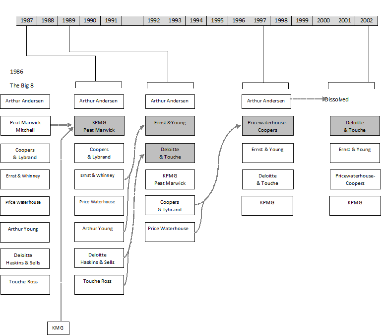
Efficiency of any audit market is broadly measured by quality of audit. Audit quality, in turn, depends on two factors- (a) ability to identify misreporting and errors in financial statements; and (b) willingness to report such errors and/or misstatements. While the first factor relies on the skill and competence of auditors, the second one surely depends on independence of auditors. It is generally believed that large audit firms can ensure better audit quality as they employ more competent resources who have requisite auditing skill as well as knowledge of select sectors or industries. Smaller audit firms could not afford large number of efficient auditors for cost reasons. As a result, audit market internationally is dominated by the oligopoly of the so-called Big 4 audit firms (Deloitte, EY, PwC and KPMG). The evolution of audit market over the past three decades showed further concentration of the industry- from Big 8 auditors to Big 4 auditors (see figure in next page). Is such a level of concentration good for the audit market? Will this feature make the audit market less efficient? Answer to these questions lies in quality of audit rendered by Big 4 and other auditors. Whether Big 4 auditors provide higher audit quality is an empirical questions and evidences are mixed. Simunic and Stein (1987) suggest that having spent heavily on building their brand names, the Big 4 auditors have an incentive to protect their reputations by providing more credible financial reports. Another study (Becker et al, 1998) shows that Big 4 auditors were able to restrain audit clients from earning manipulations. Jaggi et al (2014) confirm firms audited by industry specialists reflect a better earnings quality compared to audits by non-specialists. There are counter evidences too. Lawrence et al (2011) find that the effects of Big 4 auditors on audit quality are insignificantly different from those of non-Big 4 auditors.

The second issue concerning efficiency of audit market deals with auditor independence. Auditor tenure defines the relationship between auditor and auditee. Longer auditor tenure has mixed implications. On one hand, it allows audit firms to gain deeper knowledge about the client and thus helps the auditor ensure better audit quality. Skeptics, on the other hand, point out that longer auditor tenure creates problem with entrenchment of auditor, compromising the quality of audit. Auditor independence refers to the ability of auditors to be free from persuasion, influence or bias. One popular measure of auditor independence is the size of audit fees. Proportion of audit fees to non-audit fees is also used as a proxy for auditor independence (Frankel et al. 2002). Accounting firms argue that providing consulting services to audit clients produces knowledge spillovers that increase audit efficiency and hence questioning auditors’ independence in such situation is not valid. Others observe that non-audit fees billed to audit clients are positively associated with proxies for earnings management.

Fees capture both demand and supply factors associated with audits. However, one may question that oligopolistic premium charged by Big4 auditors may not translate to better audit quality. It is believed that auditor independence can be ensured through (a) periodic rotation of auditors and (b) regulating the type of consulting services that an auditor can render for the audit client.

Source: Patrick Velte and Markus Stiglbauer, Audit Market Concentration & Its Influence on Audit Quality. International Business Research. Vol 5, No. 11, 2012.

Audit Market in India

Audit market in India is characterized by three features- dominance of Big 4 auditor, increasing share of non-audit fee and advocacy for joint audit. Dominance of Big 4 audit firms in Indian audit market is not new. They began to grow in the Indian market since 1991 (Desai et al., 2012). However, the Big 4 multinational audit firms are not permitted to audit accounts under their own name and therefore they formed networks with local Indian audit firms to conduct audit in India (Layak & Mehra, 2009).Table 1 shows the number of companies audited by Big 4 auditors and top non-Big 4 auditors for past three financial years. The top ten audit firms accounted for audit of 36% of listed companies in NSE during 2015-16. Within the Nifty 500 subset, the dominance of Big 4 Auditors was much higher.  In financial year 2015-16, they handled a total of 234 audits (46%). The overall audit market in India is crowded with a large number of small single-location audit firms. For example, 830 audit firms audited 1519 NSE-listed companies in 2015-16 with an average volume of less than 2 auditee per auditor[1].

TABLE 1

Number of Company Audits

Note: If a client has joint audit, credit has been given to each auditor

The total audit fee paid out by companies was a significant Rs. 19,000 million[3] during 2015-16. This was an increase of 9 per cent from the Rs. 17,460 million paid out in the previous financial year 2014-15. The average audit fee paid by 1400 NSE-listed companies was Rs. 13.7 million. Table 2 shows the breakup of audit fees and total fees for last three financial years. The average audit fee earned by Big 4 auditors was Rs. 1,197 million- which was almost 90 times of average audit fees of the industry during 2015-16. There is a huge inequality in audit fee paid by large and small cap companies. About a quarter of the fees earned by Big 4 auditors came from non-audit services. Other services for Non-Big 4 auditors constitute 10% of total fees. Therefore, non- big 4 auditors are more dependent on audit fees.  Big 4 auditors in terms of business volume and fees earned dominate Indian audit market. It may be interesting to examine whether audit quality in India has improved in such a dominant audit market structure.

TABLE 2

Breakup of audit fees

Joint audit is voluntary in India. There are only 91 companies out of Nifty 500 subset practicing joint audit. Auditors in India (other than Big 4) were advocating for mandatory joint audit for large companies. However, the Government of India rejected the plea by auditors for joint audits in large companies stating that it is not a viable option for promoting domestic audit firms. Even if joint audit is mandated, it cannot be guaranteed that one small firm and one big 4 firm will handle the audit. Table 3 lists instances of voluntary joint audits of audit clients in Nifty 500 subset. About 10% of companies went for joint audit every year- these include banks and PSUs.

TABLE 3
Longitudinal distribution of firm-year observations

Compiled from Ace Equity Database.

Corporate Law and Audit Market in India

The new Indian corporate law (Companies Act 2013) seeks to address the audit quality issue from two angles- auditor rotations and prohibition in certain non-audit services to audit clients. Companies Act 2013 made rotation of auditors mandatory for listed and many unlisted companies effective from April 2017 in situations where an auditor has served in that capacity with a particular auditee for ten or more years consecutively. There is also a provision of a cooling period of five years for the audit firm with respect to the same audit client. One more important provision in this respect is about rotation of audit partner. The law states that no audit firm having a common partner(s) to the other audit firm, whose tenure has expired in a company immediately preceding the financial year, shall be appointed as auditor of the same company for a period of five years. It implies that if a signing partner of an outgoing audit firm (due to rotation) joins another audit firm, the latter audit firm will also be ineligible to be appointed as auditor of the same audit client in the immediate subsequent year. Consider an example, if Mr. X, signing partner of audit firm ABC (which has just completed ten consecutive years of audit of a client MNO) joins a rival audit firm PQR, the latter audit firm (PQR) will not be allowed to conduct audit of MNO at least for one year.  However, if MNO approaches PQR after a gap of one year since ABC audited the company, PQR would have no restriction in accepting the audit client. Therefore Indian corporate law does not specifically require audit partner rotation.

Table 4: Auditor Rotation

Auditor rotation was not mandatory under the earlier corporate law and yet it was in vogue in India (Table 4). Data on Nifty 500 over the past nine years show that annually 134 audit clients on average had different audit partners signing their financial statements (partner rotation). About 15% of the Nifty 500 companies had changed their auditor every year.

Auditor rotation is mandatory from the current financial year. Recent data on Indian audit market show that auditor rotation did not adversely affect volume of business of Big 4 multinational audit firms. For example, the top two of the Big 4 auditors in India (Deloitte and EY) have bagged enough new auditees from other two Big 4 and smaller auditors to compensate for the number of clients they lost due to mandatory audit rotation[4]. It has also been observed that large Indian corporate chose to just swap the auditors or replace an Indian auditor with one of the multinational audit firms. Therefore, the audit swap among Big4 firms also denied opportunities to local and smaller audit firms any additional business. There is no empirical evidence to suggest that auditor rotation leads to greater independence of auditors. In fact, there is greater possibility of bad audit in first year under any new auditor due to learning curve effect.

To ensure independence of auditors, another restrictive provision in the Companies Act 2013 relates to rendering of non-audit services. Services out of the ambit of a statutory auditor include internal audit, book keeping, investment advisory services, investment banking services, and management services. The restriction is much wider- it includes not only the audit client but also its holding or subsidiary companies. The term ‘management service’ is little vague and is nowhere defined in the Act. Therefore, it is not clear which non-audit services, other than taxation services, may be assigned to an auditor.  Will this restriction improve auditors’ independence? Answer is not straightforward. One obvious argument in favour of such restriction is to ensure that auditors are not dependent on corporate largesse and hence can be forthright in expressing their opinion. The ‘resource-diversion’ view suggests that expanding consulting services could undermine audit quality. There is equally strong argument against such restrictive provisions. Providing consulting services may improve audit quality- consulting staff often provide valuable insights to the audit staff because they act as ‘domain specialists’ on audit engagements.

If one puts the above two restrictive provisions – auditor rotation and prohibition of non-audit services in perspective, a natural question would be whether these provisions would have negative effect on the overall income of Big 4 audit firms.  Recent data on impact of mandatory auditor rotation in India showed that there was no reduction in audit clients of Big 4 firms due to audit swap. It is quite possible, and also perfectly legal under the new corporate law, that an audit firm retains non-audit services of a client while relinquishing audit services.  Thus, Big4 audit firms would only swap their audit clients for audit services and retain non-audit services of the old auditees. Therefore, the restrictive provisions of the Companies Act 2013 may prove to be windfall for Big 4 auditors in India.

The Companies Act did not make joint audit mandatory.  Rather the law left it to the shareholders of a company to decide about appointment of joint auditors. In case any company decides to have joint audit, the law states that the company shall follow the rotation of auditors in such a manner that all of the joint auditors do not complete their term in the same year.

References

Becker, C.L., DeFond, M.L., Jiambalvo, J. and Subramanyam, K.R. (1998), “The effect of audit quality on earnings management”, Contemporary Accounting Research, Vol. 15 No. 1, pp. 1-24.

Desai, R., Desai, V., Singhvi, M. & Munsif, V. (2012), ‘Audit fees, non-audit fees, and auditor quality: an analysis from the Indian perspective’, Journal of Accounting, Ethics & Public Policy, Vol. 13, No. 2, pp. 153–65.

Frankel, R. M., M. F., Johnson and K.K., Nelson, (2002). “The relation between auditors’ fees for nonaudit services and earnings management”, The Accounting Review, Vol. 35, No. 1, pp. 71–105

Jaggi, B., Mitra, S. & Hossain, M., (2014). Earnings Quality, Internal control weaknesses and industry specialist audits. Review of Quantitative Financial Accounting, pp. 5-32.

Lawrence, Alastair and Minutti-Meza, Miguel and Zhang, Ping, Can Big 4 Versus Non-Big 4 Differences in Audit-Quality Proxies be attributed to Client Characteristics? (June 16, 2010). Accounting Review, Vol. 86, No. 1, pp. 259-288.

Layak, S. & Mehra, P. (2009), ‘Inside the secret world of auditing’, Business Today, 22 February, pp. 54–60.

Simunic, D. A., and M. T. Stein. (1987). Product differentiation in auditing: Auditor choice in the market for unseasoned new issues. Canadian Certified General Accountants’ Research Foundation, Vancouver, B. C.

[1] Prime Database, September 2016

[2] Big N Audit Groups as per Prime Database: 1. Deloitte Group (Deloitte Haskins & Sells, Deloitte Haskins & sells LLP, A F Ferguson & Co, C C Chokshi & Co, Fraser & Ross, S B Billimoria & Co) 2. EY Group (S R B C & CO LLP, S R Batliboi & Associates LLP, S R Batliboi & CO LLP, S V Ghatalia & Associates LLP) 3. Price Waterhouse Group (Price Waterhouse,Price Waterhouse & Co, Price Waterhouse & Co LLP, Bangalore, Dalal & Shah, Lovelock & Lewes) 4. KPMG Group (B S R & Associates LLP, B S R & Co LLP,B S R & Company, B S R and Associates, B S R and co, B S R and company)

[3] Data based on 1,389 companies for which audit fee/total fee data was available. Source: Prime Database

[4] The Economic Times, June 14, 2017

Credit Default Swaps (CDS) are financial derivatives that earned the notoriety of being characterized Financial Weapons of Mass Destruction in the aftermath of the 2007-8 financial crisis, which originated in the US. CDS is a kind of insurance against credit default. It was issued by insurers like AIG and other market participants, and bought by investment banks like Goldman Sachs, to protect their investment in subprime and other securities. Speculators too can buy the contract without holding the underlying security. When the financial crisis reached its climax, AIG nearly went down the Lehman Brothers route to bankruptcy thanks to its CDS exposure. It avoided Lehman’s wretched fate with the US government’s rescue, but it was a close call. At its peak, the total outstanding CDS contracts in the market was estimated at more than 60 trillion dollars, bearing no correlation to the underlying value of the securities it sought to protect. An implosion in the CDS market, given its size, could have sounded the death knell of the financial markets, hence the tag Financial Weapons of Mass Destruction for these swap contracts.

Since the winding down of the crisis days, CDS no longer attracts the same level of attention, though the market for the swaps continues to be active.

Basel Committee Standards

Prior to the crisis, the Basel Committee for Banking Supervision had published two accords for capital adequacy, the Basel I standards in 1988 and Basel II in 2004. Basel 1 was a simplistic approach. It painted all counterparties in a particular category with the same brush by assigning a uniform risk weightage. Emphasis was on credit risk. Basel II accord proposed a more risk sensitive approach towards capital adequacy measurement. It also introduced capital standards for operational risk and incorporated the market risk measures brought in, post the Basel I accord. The Basel II accord was an abysmal failure in addressing the systemic, liquidity, leverage and pro cyclical issues in the banking sector, which led to and exacerbated the financial crisis.

The Basel III Accord

The Basel Committee, learning from these lessons, introduced several measures including a leverage ratio that sought to constrain excess leverage in the banking system, and global liquidity standards, along with a framework to promote the conservation of capital and the build-up of adequate buffers above the minimum that can be drawn down in periods of stress.

A critical lesson learnt from the crisis was the need for an additional capital layer that can absorb losses on a going concern basis.

The earlier Basel accords had elements of such capital but they could not act as an effective layer for absorbing losses for the simple reason that they were structured to do that only on a “gone concern” basis i.e. in a liquidation scenario. Depositors would have to stand in a queue and wait for liquidation of the assets of their bank to recover their investments. Such a “forced sale” usually results in lesser valuation of assets and takes time.

AT1 Bonds a.k.a Perpetuals

Basel III accord therefore introduced a new instrument, the Additional Tier 1 (AT1) bond, to protect depositors of a bank on a “going concern” basis. The essential element of this instrument is the imposition of losses on its holders without the bank being liquidated, if the Common Equity Tier 1 (CET 1) ratio falls below a threshold level. The bonds are also known as perpetuals as they do not have a specific redemption date. To qualify as an AT1 bond, 14 criteria are specified by the Basel Committee, the following being noteworthy apart from the perpetual nature:

• Callable at the initiative of the issuer only after a minimum period of five years. For exercise of a call option, a bank must receive prior supervisory approval
• The bank must have full discretion at all times to cancel distributions/payments of coupon/dividends
• Coupon/dividends must be paid out of distributable items
• Principal loss absorption through either
• Conversion to common shares at an objective pre-specified trigger point or
• A write-down mechanism which allocates losses to the instrument at a pre-specified trigger point.

AT1 bonds are quasi equity instruments that seek to protect depositors through the loss absorption mechanism and discretion on coupons, while leaving investors in the bonds in high risk circumstances.

Why would an investor go for AT1 Bonds?

The answer can be summarized in a single word: yield.

Scenario in today’s yield starved world:

(as on 8th September 2017)

In comparison, AT1 bonds stand out, with bonds of top rated global banks offering around 5%.

Indian PSU banks yield to maturity on rupee perpetuals ranges between 8 pct and 12.5 pct. The investors in AT1 bonds are primarily institutional. Regulators generally discourage the small retail investor from this segment. It is the expectation that wholesale investors with “superior” credit risk and market risk assessment skills are better equipped to invest in such bonds.

Another perplexing factor in AT1 bonds: why would someone invest in a bond that does not ever repay its principal? The call option comes to the rescue here. Despite issuers being explicitly prohibited under the Basel standards from creating an expectation with investors that the call will be exercised, the markets expect banks to call the bonds at the end of 5 years and usually well capitalized banks oblige. Voila! A perpetual bond is now a very attractive short term instrument with a mouthwatering yield.

Are AT1 Bonds serving the purpose?

Earlier this year, Banco Popular of Spain faced mounting losses and a run on the bank by its depositors. In a deal orchestrated by the European Commission, the larger Spanish bank Santander, took over Banco Popular, while imposing a write-down on AT1 bond holders for nearly 2 billion Euros. In the rescue of the Italian bank Montei Dei Paschi, 4.5 billion euros were converted into ordinary shares, though retail investors were spared.

The recent instances broadly prove that AT1 bonds are working as intended, though some central banks question if the write-downs happened at the European banks only when the banks were on the verge of becoming a “gone concern”.

The experience with weak public sector banks in India offers a study in contrast. The Indian government’s apparent willingness to support its subsidiary banks through additional capital to prevent an AT1 bond write-down, is perhaps a reflection of its worries of a contagion risk to the banking system and its own credibility in the traditional role of a promoter.

Moral hazard

The regulator now requires banks to provide for 50% of outstanding secured loans as soon as a defaulter is referred to the National Company Law Tribunal (NCLT) under the Insolvency and Bankruptcy Code, and 100% if the defaulter goes into liquidation. PSU banks in India, with large problem loan exposures being referred to the NCLT for resolution, would therefore require significant amounts of additional capital in the near future to meet the standards for CET 1 ratio as per the Basel III accord. This ideally should happen through the write-down of AT1 bonds, unless the government continues to step in with its own capital infusion. Apart from fiscal constraints that the government faces, such large scale bail out of institutional holders who have been enjoying high returns on account of the risky nature of AT1 bonds, will entail a moral hazard. It also goes against the very raison d’etre of the AT1 bonds which entails holders absorbing losses. The US government bailout of Wall Street Banks during the financial crisis attracted scathing criticism that it was tantamount to private profits and socialized losses. In a developing country like India, a tax payer led bailout of institutional investors in AT1 bonds, may not be politically palatable.

The concerns around protection of the principal portion of the AT1 bonds apart, the risk of nonpayment of coupon remains. Basel standards allow coupon (interest) payment only from distributable reserves. Further loan loss provisioning by weak PSU banks could lead to reserves being wiped out and trigger a default on coupon payments. Capital infusion by the government can potentially bailout the principal portion of AT1 bonds but cannot support banks without reserves in meeting coupon payment obligations.

The next Financial WMD’s?

A final word on the potential of AT1 bonds to wreak havoc in the global financial system from a systemic perspective. An AT1 bond write-down for institutional holders could very well trigger a run on the bank by retail depositors who may fear that they may be next in the line to take a hit. As long as the problem is localized as observed recently in Spain and Italy, there is no risk to the broader banking system. But en masse write offs of AT1 bonds at multiple banks in the event of a scenario like the last financial crisis is a real possibility. If depositors stampede to the exits, the inter connected banking system would again be at risk as witnessed during the dark days of 2007-8.

Governments, regulators and financial market participants can perhaps take comfort from the recent statement of Janet Yellen, the Chairperson of the Board of Governors of the US Federal reserve, that she does not foresee another financial crisis in our lifetime. Let’s hope that she is right! Readers may however take note that she did appear to back track on her remarks in a subsequent testimony to the US Senate.

Traditional view on OTC derivatives risk

Until 2008, OTC derivatives focussed on market risk. Counterparty risk was considered secondary. Most counterparties had strong credit rating and the possibility of default was seen as remote. While Basel-II introduced a capital charge for counterparty risk in the trading book and accounting rules introduced in 2006 required counterparty risk to be factored into balance sheet valuations, it continued to be managed at PFE (Potential Future Exposure) level.

Derivatives were valued using the concepts of risk neutral probabilities and no arbitrage. A risk neutral portfolio is expected to earn a risk-free rate and LIBOR rates were the benchmark. The “risk-neutral” or “risk free” price assumed a credit risk free world – where none of the counterparties would default and all contractual cash flows will happen

2008 financial crisis

A cascade of defaults in 2008 (Lehman in particular) exposed the weakness of this traditional view.

Financial institutions and regulators realized that any firm could default and that they had to put much more emphasis in understanding, managing and controlling counterparty risk.

Historically, LIBOR was viewed as the risk free rate, as it was close to AA-rated interbank loans. Post Lehman’s default, the 3-month Fed funds-LIBOR spread widened to 350bps – calling into question the use of LIBOR as benchmark rate. Subsequently, the overnight index swap (OIS) rate has become the “risk-free” rate ¹.

The assumption of no defaults proved to be unrealistic in the post –Lehman world. Financial institutions realized the need to adjust the risk-free price by an amount equivalent to the market price of the counterparty risk embedded in the derivative contract.

Presently, CVA (Credit or Counterparty Value Adjustment) has become very important for financial institutions and they devote substantial resources to calculate CVA in their derivative book. It has been reported that during the 2008/09 financial crisis, two-thirds of the credit related losses that banks suffered were CVA related (paper losses on the balance sheet), as opposed to actual default losses. Once counterparty risk (CVA) is priced, the bank can decide whether to monetize that risk (continue to carry that risk and expect that not too many counterparties will default) or hedge it.

Credit Value Adjustment (CVA)

CVA is an adjustment to the “risk-free” value of a derivative to account for potential counterparty default.

P_{Risky value} = P_{Risk free value} – CVA … (1)

P_(Risky value)=Price of derivative after adjusting for counterparty risk
P_(Risk free value)=Price of derivative without counterparty risk (OIS discounting)
CVA=Couonterparty credit risk adjustment

Historically, CVA was seen as a “credit charge” for pricing and a “reserve” or “provision” for financial reportingpurposes². More recently, CVA is defined as the price of hedging out the counterparty risk, irrespective of default

¹ For example the Fed funds rate in USD – the interest rate at which depository institutions lend balances at the Fed Reserve to other depository institutions overnight. It is considered safer than unsecured deposits (LIBOR loans) because it occurs in the Federal Reserve System under the oversight of the Fed.

² While this doesn’t represent the actual loss for a trade, it’s sufficient in a portfolio context assuming there are many trades across different counterparties 

CVA formula

CVA ≈ −LGD ΣB (ti) × EE (ti) × PD (ti − 1, ti)

LGD (Loss given default)= percentage of exposure expected to be lost if the counterparty defaults

B (ti) = risk free discount factor at time ti. Any future losses  must be discounted back to current time

EE (ti) = Expected exposure for the relevant future dates, ti

PD (ti − 1, ti) = Marginal default probability in the interval between (ti-1) and ti

CVA can be expressed either as a standalone value or as a spread (per annum charge).

Example – CVA components for a swap trade

While it can be computed for individual trades, what matters is the CVA of a netting set. This is important because the price of counterparty credit risk needs to mimic what will happen if a counterparty defaults. When the counterparty defaults, the Master Agreements between counterparties will legally put together trades that can be netted off for the liquidation of the portfolio and drive the subsequent payments to and from the defaulted firm. An individual trade should be evaluated only in terms of its contribution to the overall CVA of the netting set.

Debt Value Adjustment (DVA) and Bilateral CVA (BCVA)

CVA assumes that the counterparty making the calculation will not default. International accounting standards allow an institution to consider its own default, while valuing its liabilities. Accordingly, the liability component of credit exposure (negative exposure) can be included in the pricing of counterparty risk, as debt value adjustment (DVA)

Bilateral CVA means that an institution will consider its own default, while computing CVA. In the bilateral model, the adjustment to the risk-free value of a derivative is given by

BCVA = CVA + DVA ….(3) where CVA is a cost and DVA is a benefit

Data challenges

Obtaining the necessary market data is a common challenge in CVA computation, especially the default probability and expected exposure components.

CVA computation requires risk neutral probabilities of default. IFRS 13 requires entities to make maximum use of market-observable credit information. CDS spreads may provide a good indication of the market’s perception of counterparty’s creditworthiness. However, many counterparties are “illiquid credits” with no direct market observable measure of creditworthiness. There is a significant subjectivity in obtaining default probabilities for illiquid credits. An even more difficult task is estimating correlations, between market risk factors and credit spreads. These correlations are important in order to be able to model wrong way risk

Exposure quantification is quite difficult over long horizons given the increasing uncertainty about market variables

Regulation and Capital requirements

Basel III rules were introduced in 2009 to strengthen bank capital bases and introduce new requirements on liquidity and leverage. A large portion of the Basel III changes relate to counterparty credit risk and CVA

A capital charge was introduced for CVA volatility (CVA VaR), in addition to the existing charges against counterparty credit risk. This has arisen because a large proportion of the counterparty credit risk related losses in the financial crisis were seen as being mark-to-market based (CVA) rather than due to actual defaults, which were the focus of the Basel II regulations. This had some unintended consequences.

The regulatory focus on CVA seemed to encourage active hedging of counterparty risk so as to obtain capital relief. However, the CDS transactions that were most important for such hedging (single-name and index OTC instruments) introduced their own form of counterparty risk, in particular the wrong way type. The CDS market is even more concentrated than the overall OTC market and has become less, rather than more, liquid in recent years. Since it was the new CVA capital charge that was partially driving the buying of CDS protection that in turn was apparently artificially inflating CDS prices, the methodology for the additional capital charges for counterparty risk has been questioned.

SEBI redeemed itself on 4^th August, 2017. This it did by issuing a circular which mandated listed companies to report ‘default’ in servicing bank loan, within 24 hours of the default. The circular which will become effective on 1^st October 2017, a day before Gandhi Jayanti, would go a long way in enhancing the level, quality and urgency in disclosures to investors in Indian markets. As such, the markets have to make do with much inferior quality corporate disclosure than is the case is more developed markets.  The circular unambiguously defines default as ‘non-payment of interest or principal amount in full on the pre-agreed date”. That the globally accepted definition of default would come from market regulator, and not the banking regulator, is a thought provoking matter in itself.

This mandate from SEBI will go a long way in reducing the likelihood of another corporate credit blow-up, on the lines India is currently experiencing. However, this had come in 2011, it might have prevented at least INR 4 lakh crore shareholder value erosion which happened in the following six years. While SEBI may have redeemed itself the same cannot be said about the Board Members of NPA companies. The Board particularly the independent member, of over 500 listed and defaulted companies, have still to answer to their shareholders whether they have been doing their job at all or not.

Board members, particularly independent members, usually are experienced individuals with expertise in fields such as accounting, legal, banking, economics or business. Most of them are expected to know that in the event of a payment default the company’s equity value technically becomes negligible, if not zero. The debt holders have economic and legal claim (in most countries and now also in India) to the assets of such a defaulted company thereby causing the equity holders’ stake ie;stock price to crash. As the information of default ‘leaks’ out into the market the share price nose-dives. From the time a company moves to an NPA or acknowledged default state typically stock price erodes by 95% to 99% of pre-default peak price.

 The board member had ample opportunities and examples from Indian markets about stock price crash of defaulted companies. Thus they can clearly figure out the supreme importance of information about delinquency status of the company and how valuable the information is to minority shareholder. It is not too much to expect that board members may have figured out that ‘default’ on any debt is a material event from the perspective of the shareholder. Now that SEBI has issued the circular and expect compliance from 1^st October 2017, we still do not see companies under the aegis of their board members proactively reporting to exchange about their delinquency status. Of course it may be a case that none of the companies in India are currently in stage of unacknowledged default, but given the economic situation this appears less likely.

Are Board Members of NPA Companies Negligent?

Indian regulators, thus far, have been behind the curve in terms of creation of rules which reduce information asymmetry with respect to investors and minority shareholders of the company. It may not have been so much an intent issue but possibly a lack of appreciation of the importance of ‘default’ information to shareholders.

In the original Listing Obligation and Disclosure Requirement (LODR), a listed company was expected to share information about material events ranging from disruptions of operations due to calamity, commencement of commercial productions, litigation, organisational restructuring, issuance or forfeiture of shares, non-payment of dividend and the like. These are clearly material events but it is arguable whether any of them can erode shareholder value by 95% to 99% the way a corporate default does. To be fair to the board members of defaulted companies the fact that any default on financial obligation is a material event for the company has not been on top of mind of both the market regulator as well as the banking regulator prior to 2015.

 In the earliest versions of LODR, reference to default of payment on financial obligations was absent. Gradually, non-payment of dividends was introduced as an event requiring disclosures, subsequently default on redemption of hybrid instruments such as foreign currency convertible bonds (FCCB) was identified as an event requiring disclosures and more recent inclusion was default on listed debt instrument such as Non-Convertible Debenture (NCD). Strangely, a time period was not specified other than the requirement that the news is to be shared with the exchange ‘promptly’.  Even when such defaults happened it was more often via a news leak that investors got information about default events and only thereafter would the company inform the exchange.

But then the original version of listing agreement did contain a clause which read “The company should ensure timely and accurate disclosure on all material matters including the financial situation, performance, ownership, and governance of the company”.  That none of the independent directors, pushed a company to proactively disclose event of default on any debt obligation may be a comment on the maturity of all market participants which include regulators, institutional investors, retail investors , market commentators and of course the Board Members. The 4^th August 2017 regulation of SEBI possibly underscores the fact that unless pushed, the market forces by themselves may not push most Indian companies, in general, to adopt world class disclosure norms and governance practises.

Did the Management and Board Neglect the September Wakeup Call?

 On September 2015, SEBI enhanced the LODR to provide further regulatory clarity on the responsibilities of the Board and Key Management Personnel (KMP) with respect to disclosure of information to the exchanges. An argument can be made that Board Members and KMPs of defaulted companies may not have been complying with this regulation in spirit and possibly also in letter, when they did not share the information of a default/delinquency event to the exchange. Let’s get into the details of this argument by focussing on responsibilities of the board members, interpretation of materiality and access to information.

The enhanced LODR specifically articulated the responsibilities of the board . The prominent ones are the following:

-The board of directors and senior management shall conduct themselves so as to meet the expectations of operational transparency of stakeholders while at the same time maintaining confidentiality of information in order to foster a culture of good decision-making.

-Ensuring the integrity of the listed entity’s accounting and financial reporting systems, including the independent audit, and that appropriate systems of control are in place, in particular, systems for risk management, financial and operational control, and compliance with the law and relevant standards.

– Overseeing the process of disclosure and communications.

Here one may argue that not disclosing event of default due to non-payment of bank loans does not speak highly of operational transparency and reflects poorly on integrity of reporting system with respect to risk management and financial control.

Arguably, there was a enough clear guidance in the September 2015 regulation which may have prompted a prudent board to report a default in payment of bank loan to the exchange. Further there was an a more overarching requirement  which requires  “Every listed entity shall make disclosures of any events or information which, in the opinion of the board of directors of the listed company, is material.”  Further the regulator  provided guidance for determination of materiality of events/information.

Two points that  highlight what may constitute a material event:

(a) the omission of an event or information, which is likely to result in discontinuity or alteration of event or information already available publicly

(b) the omission of an event or information is likely to result in significant market reaction if the said omission came to light at a later date;

The company management and the board members clearly know that information on ‘event of default’  on financial obligations always cause quite violent market reactions leading to sharp correction in the stock price. It beats conventional logic on why the  board members refused to identify non-payment of bank loans as a material event requiring disclosure to stock exchange.

Of course, some may point out that the Board Members may not have access to information on whether the company was defaulting on payment of bank loans. Here it may be mentioned that among the mandatory list of minimum information that is supposed to be placed before the board of directors, the disclosure on “any material default in financial obligations to and by the listed entity, or substantial non-payment for goods sold by the listed entity “  is loud and clear.

So if the management is not placing the default information to the board, the KMP is violating the LODR.

Selective Bouts of Investor Activism Does Not Help

It is a surprise that despite Company’s Act 2013 allowing for filing of class action suits by the shareholders none of the present NPA companies or their boards has been sued for negligence in duty or non-disclosure of material information such as those related to default which caused shareholders to lose massive wealth in stock market. Clearly institutional investors, corporate governance firms as well as informed individual investors have missed to highlight this massive and widespread lapse of corporate governance. As such, in most instances, Indian investing community wakes up to only those instances of corporate governance violations where the violations are disclosed by disgruntled promoters themselves! It is surprising that while everything from policy paralysis, to bank’s over lending to corporates, to global commodity price moderation, has been blamed for the Indian credit blow-up, this significant lapse in duty of the Board members of such defaulted company has not been highlighted.

The rising corporate debt and higher default rates have led to a continuous increase in distressed loans in Indian financial system. The situation worsened when stressed asset ratio rose from 7.6 % in March 2012 to 11.5 % in March 2016 and further to 12% in March 2017. As of June 2016, the total amount of Gross Non-Performing Assets (NPA) for public and private sector banks was around Rs. 6 lakh Crore (almost $10 billion). Alarmed by the deteriorating asset quality, the Reserve Bank of India (RBI) in April 2015 had urged all commercial banks to put in place an early warning system to prevent financial fraud. In March 2016, the Securities and Exchange Board of India (SEBI), the Ministry of Corporate Affairs (MCA) and the Institute of Chartered Accountants of India (ICAI) had emphasised the need for developing an early warning system aimed at zeroing in on companies that have taken funds from public and whose balance sheet parameters show that they may renege on repayment. The problem with this approach –generating early warning signals from financial statements- is it may lack predictive power. This would be particularly true for firms which ‘window dress’ their financial numbers to ‘defer’ release of bad news. Lenders typically concentrate largely on financial parameters at the time of loan origination and subsequently track the behaviour of borrowers through financial statements and other financial data furnished by the borrower. However, the information in the financial statements may not reveal the actual state of affairs of a borrower. Take the following example (Table 1). These three companies defaulted in 2015. Their financial health did not show any sign of trouble/irregularity three years (2012) before the year of default. In fact, leverage (debt-equity) of two companies was much less than one. Operating profit margins were in double-digit for two firms. The Altman’s Z-score[1] was much above the comfort zone for all the three companies in 2012. One might point out that the EMS can predict distress one year ahead and not so early. However, even in the year of default (2015), the EMS was above 2.6 for all three companies.

Much of the research has so far explored the relationship between financial distress and historical accounting information. However, the quantitative financial information comprises only approximately 20% of all the information contained in annual reports (Beattie et al. 2004). Therefore to obtain a complete picture of financial health of a company, it is necessary that one uses the qualitative information provided in corporate annual reports. There is of late a growing interest among finance and accounting research community in analysing and quantifying the qualitative information present in annual reports. Loughran, McDonald ( 2011 ) analysed the tone of corporate annual reports (sentiment) and observed that sentiments expressed in annual report text data is significantly correlated with profitability, trading volume, and unexpected earnings for listed companies in USA.

Table 1: Financial Health of Three Companies

Realizing the need for greater scrutiny of annual reports, the RBI[2] instructed banks to undertake a detailed study of the Annual Report, and not concentrate merely on financial statements. At present detection of loan frauds takes an unusually long time, which may delay action against any fraudulent entity causing huge losses to financial institutions. So, early detection of any trouble or distress of borrowers would really help in controlling the menace of non-performing assets. The lenders in India should learn the art of extracting information from large text documents and improve their present rating system by supplementing financial parameters with text-based information. This would make the existing rating system more robust.

We have observed, after manually going through hundreds of annual reports of corporates, firms reveal more in the ‘text’ part of the annual report. Companies, more so the listed ones, become careful while presenting financial statements simply because this section of the annual report is scrutinised most by analysts, investors and lenders. We have developed a proprietary text-based model for estimating default probability of firms and we claim that our model has much better predictive power than Altman’s. Our proposed model is equally effective in case of unlisted firms. Further our text-based model is designed to capture any kind of trouble or uncertainty that a firm faces in addition to default risk.

Words reveal more

Our model is developed using text present in the annual report of a company. We have only used three sections of an annual report- Directors Report (including Management Discussion and Analysis), Audit Report and Notes to Accounts. It is important to note that annual report (except the audit report) is a self-report of a company and hence such a document is bound to have strong bias. Yet we were amazed by the quality of information that one can extract from such a biased text. Let us take the case of Vijay Textile (mentioned in Table 1). The company reported an operating margin of more than 28% in 2012 with a debt-equity ratio of less than 1.5. Even in the year of default, the debt-equity did not cross 2, though the sales growth was negative. However, if one looks at the annual report of the company over past few years prior to the year of default, one would notice that the company had started facing financial hardships at least four years before 2015 (Table 2). It is interesting to note that the Altman EMS improved over the years whereas the text of annual reports clearly showed that the firm was burdened with huge financial hardship so much so that the company had to dispose of some assets way back in 2011. The firm witnessed inventory pile up and lower profitability in 2012 and the situation did not improve thereafter leading to huge pressure on liquidity in 2014. The material information captured in the text of the annual report, in this example, proves that it makes economic sense to analyse the non-financial information as seriously as one does for financial information. We find that directors report provide most of material information and audit report provided least marginal information.

Magnusson et al. (2005) use self-organizing maps to visualize the changes in the writing style of the annual reports of telecommunication companies. They observed that when a company is expected to perform well, the tone of the report remains positive with extensive use of optimistic vocabulary as compared to a less optimistic and more conservative tone when expecting worse financial performance.

Table 2: Excerpts from Annual Report

Methodology Explained

Each piece of annual report text data provides one aspect of reality about a firm’s condition for a particular financial year. But the text data contains a lot of noise or irrelevant information, which makes extracting only useful information, using computational tool, a bit cumbersome. So text data cleaning is a first important task before performing any analysis on it.

For cleaning the dataset, we have used the following steps:

1. Remove all hypertext data, urls etc.
2. Remove the selective dash only like un-relalistic is converted to unrealistic, un-certain to uncertain but not profit-loss to profitloss, rather profit loss. We identify the selective prefixes which changes/add stress on the only desired sentiment of words.
3. Remove all non informative text data like numbers, dates, serial numbers for starting points, comma, dots, anything between () or {} or [].
4. Remove all phrases which are general accounting literature terms like profit and loss, gain and loss, all words in capital letters.
5. Perform the lemmatization of the keywords to remove inflectional endings only and to return the base or dictionary form of a word, called lemma. e.g. diminish , diminishes, diminishing, diminished reduced to diminish.
6. Remove all stop words. There is a list of around 4000 words mainly consisting of objective words which are common literature words and possess no sentiment. This stop word removal greatly helped in inferring the results.
7. The negation words change the overall sentiment of word used in a sentence. So the negation marking is done to correctly infer the actual sentiment expressed by a human writer.

We have used ‘bag of words’ approach in extracting sentiments out of text. A text document is converted into a vector of counts. The vector contains an entry for every possible word in vocabulary. The original text is a sequence of words but bag-of-words has no sequence. It just remembers how many times each word appears in the test. A matrix can represent the corpus of documents with one row per document and one column per feature (e.g. word) in the corpus (popularly known as term-document matrix). The element (i,j) within this matrix represents term frequency of feature in document. The resultant representation is called bag-of-documents representation. The final words list extracted from annual reports text using statistical feature selection methods is not exhaustive. The human intervention is desired. So finance and accounting expert intervention helped us create an exhaustive list of features (words) which may be generalized to all annual reports, e.g. qualified if used in auditor’s report carries a negative sentiment but in general English dictionary it is a positive sentiment word. The expert judgments helped in categorizing the exhaustive list of keywords into most probable sentiments associated with the feature in finance and accounting literature. The feature selection process reduced the number of keywords by 98%.

The process of feature selection has started with initial corpus of 50 distressed and 50 non-distressed firms. With initial inferences, iteratively the corpus is increased to around 800 firm’s annual reports for time period 2007-2015, representing different sectors and belonging to either of one category i.e. distressed or non-distressed firms. We have finally created two important bags of words- fear and sunshine. Fear word list consists of all the constraint words used in finance and accounting literature for disclosing the current or anticipated hardship. Sunshine word list consists of all the word used by managers for disclosing positive information in the annual reports[3]. We have used several metrics for measuring sentiments (Table 3).

Table 3: Sentiment Metrics

* Total number of words in the document. DI stands for Distress Intensity

Results

Our sample consisted of annual reports of both public and privately held companies operating and registered in India. We have selected the companies functioning in around 36 different sectors. Due to special nature of business and financial structure, insurance and banking firms were excluded from the sample. Our final sample consisted of 780 companies divided almost equally between financially distressed and healthy firms. The descriptive statistics of fear and sunshine words (Table 4) show that these words have discriminating ability between distressed and non-distressed firms. Average number of negative words (fear score) has increased for both financially distressed and healthy firms over the years. Surprisingly the optimism (sunshine words) in the Indian corporate sector has declined during 2007-2015. The fear score is high for financially distressed firms as compared to their sunshine score. Similarly for non-distressed firms the sunshine score is comparatively higher than their fear score.

Table 4: Descriptive Statistics of Bag of Words

Our results show that text–based model performs better than Altman Z-Score in predicting default (Table 5). Panel A of the table shows that our text-based model has better predictive power than Altman’s EMS. For example, our model could correctly classify 83% of distressed firms two years before the year of default where the Altman’s EMS could classify only 44% correctly. One may wonder why our model wrongly identifies a third of healthy firms as distressed firms. The reason is our model captures any kind of trouble and not necessarily financial distress.

Table 5

Panel A: Percentage of firms identified as distressed using Text of Annual Report

Panel B: Percentages of firms identified as distressed using Altman EMS

We have also tried to map the default probability with firm ratings. We have used latest available rating of long-term debt instruments (or loans) issued (raised) by firms in our sample. Information on ratings were available for only 653 out of 780 firms in our sample. We observe that text-based probability estimates are highly correlated with the ratings of firms.

Table 6: Credit Ratings and Default Probabilities

PD implies Probability of Default. NM=Not Mentioned. WD= Rating Withdrawn

The focus of the study was to design an early warning measure of financial distress based on qualitative information present in corporate annual reports. We set out to construct a systemic financial distress prediction process based on the tone of corporate annual report text information and proposed a measure to quantify both positive and negative sentiments in the annual report’s language without using any accounting information. We turn to the case of Vijay Textiles for the last time (Figure 1). As mentioned earlier, the company defaulted in 2015 and Altman’s EMS failed to capture the phenomenon. However, our ‘fear score’ surpassed ‘sunshine score’ in 2011 and thereafter the ‘fear score’ was always higher than the ‘sunshine score’. Also the probability of default was close to 60% in 2011 and increased further thereafter.

Figure 1: Vijay Textiles: Probability of Default Estimates

The proposed sentiment based method performed better than the traditional accounting information based models for predicting the probability of distress. Hence, it is harmful to ignore the boring text of an annual report.

[1] The Altman Z-Score is used as a tool for analyzing the level of distress a firm might face in next one year. Altman et al (1995) introduced a revised Z-score model for the non-manufacturing and manufacturing companies operating in developing countries using the sample of Mexican Companies. They called the revised model as EMS (Emerging Market Score). The present study uses the EMS. Any firm, which secures an EMS of 1.1(2.6) or below (above), has high (low) risk of default.

[2] Framework for dealing with loan defaults, June 2016

[3] We regret our inability to further describe the methodology due to its proprietary nature.

References:

Altman, E., Hartzell, J., Peck, M., (1995). A Scoring system for emerging market corporate bonds. Salomon Brothers High Yield Research. June.

Beattie, V., McInnes, W., & Fearnley, S. (2004). A methodology for analysing and evaluating narratives in annual reports: a comprehensive descriptive profile and metrics for disclosure quality attributes. Accounting Forum, 28 (3), 205–236.

Tim Loughran and Bill McDonald (2011), When is a Liability not a Liability? Textual Analysis, Dictionaries, and 10-Ks. Journal of Finance, 66 (1), 35-65

Magnusson, C.; Arppe, A.; Eklund, T.; Back, B.; Vanharanta, H.; Visa, A. (2005). The language of quarterly reports as an indicator of change in the company’s financial status. Information & Management, 42 (4), 503-53

The RBI has released an important and timely discussion paper on April 4 2017 on the “Wholesale and Long-Term Finance” (WLTF) Banks.[1] This is in consonance with announcement made in the first Bi-monthly Monetary Policy Statement 2016-17 (of April 5, 2016) which had mentioned that the RBI would “explore the possibilities of licensing other differentiated banks ….and had identified custodian banks and banks concentrating on whole-sale and long-term financing, as two other classes of differentiated banks”. Looking into cross-country experience, the present RBI proposal views extends that vision WLTF banks that would focus primarily on “lending to infrastructure sector and small, medium & corporate businesses.” What is their genesis? Are these WLTF banks going back from the professed path of financial sector reforms whereby development banks like IDBI or ICICI banks were winded up? This short piece makes a speculative attempt to look into some such questions.

Genesis and Functions

As far as the genesis of WLTF banks is concerned, it can be traced in the Report of the RBI Committee on Comprehensive Financial Services for Small Businesses and Low Income Households (Chairman: Dr Nachiket More; June 2014) that envisaged a class of differentiated banks called “Wholesale Banks”.[2] It noted:

“Given the enormous cost and informational disadvantages that National Banks face in India it is possible that this may be an entirely acceptable and even a preferred strategy for a large, systemically important bank to follow, …. so that it is able to maintain an extremely high level of safety in its credit ratings and can therefore act as a high quality aggregator of both deposits and loans allowing smaller and more specialised banks and financial institutions to transfer their own systematic exposures to such a Wholesale Bank.”

            Taking a cue from the Mor Committee Report the April 2017 proposal of RBI has noted, “The Wholesale and Long-Term Finance (WLTF) banks will focus primarily on lending to infrastructure sector and small, medium & corporate businesses. They will also mobilize liquidity for banks and financial institutions directly originating priority sector assets, through securitization of such assets and actively dealing in them as market makers” (p.10).  It may be useful to note the following specific features of these WLTF banks:

1. Activities: The primary activities of WLTF banks will be deposits or loan products for wholesale clients and financing of infrastructure sector and core industries. These banks also act as “market-makers in securities such as corporate bonds, credit derivatives, warehouse receipts, and take-out financing etc” and will provide refinance to lending institutions. These banks may also offer investment banking services related to equity / debt investments and forex / trade finance. But unlike investment banks these services will be of ancillary interest to WLTF banks.
2. Sources of Finance: Primary sources of funds for WLTF banks could be a combination of “term deposits, debt / equity capital raised from primary market issues or private placement, and term borrowings from banks and other financial institutions”.
3. Deposits: These banks may be permitted to accept deposits only “above a large threshold amount” and are expected to have negligible retail segment exposure. Deposits of these banks will have deposit insurance cover.
4. Regulatory Requirements: These banks are expected to have a higher level of initial minimum paid-up equity capital, say Rs. 1,000 crore or more. While these banks may be required to maintain CRR they would be eligible for exemption from CRR requirement for the liabilities under infrastructure bonds. Finally, some relaxation in respect of prudential norms on liquidity risk (e.g., Liquidity Coverage Ratio / Net Stable Funding Ratio) may be considered for WLTF banks. Opening of rural and semi-urban branches and compliance to priority sector lending norms would not be mandated for these banks

The Rise and Fall of Development Banks in India

But why does a country need WLTF banks? Are these not look-wise quite similar to the development banks? It is useful to turn to Nayyar (2015), who said:[3]

“The economic logic of development banks is simple. In countries that are latecomers to industrialisation, capital markets are imperfect. Therefore, new firms, which seek to enter the industrial sector, find it exceedingly difficult to obtain finance for their initial investment….. The problem is exacerbated when such investments are characterised by lumpiness and returns accrue only after a gestation lag. In these circumstances, firms might underinvest, or fail to invest, in the creation of manufacturing capacities that require learning capital. … The problem is far more acute for long-term finance where there are indivisibilities in the capital needed by new firms, as the initial losses are high and the learning period is long. …. Latecomers to industrialisation create development banks essentially to meet these financing needs of pioneering firms in a non-existent or infant manufacturing sector, which are not met by capital markets or commercial banks because, in their calculus, the risk is too great” (p.51; emphasis added).

It may be useful to get a historical perspective of development banks here. India’s first development bank, the Industrial Finance Corporation of India (IFCI) was set up in 1948. Within next five years, a number of state governments with the encouragement of the central government set up their own State Financial Corporations (SFCs).  Later in 1954 the National Industrial Development Corporation (NIDC) was set up as an agency of the Central government to provide both entrepreneurship and finance to the industrial sector and functioned till early 1963.  The Industrial Credit and Investment Corporation of India (ICICI) was floated as a public limited company with initiatives of the World Bank, the Government of India and representatives of Indian industry. While its primary objective was to provide medium-term and long-term project financing to Indian businesses, it emerged as the major source of foreign currency loans to Indian industry as well as for doing underwriting for the Indian corporates. Subsequently in 1964, the Industrial Development Bank of India was set up as an apex institution in the sphere of medium- and long term finance. It took over the business of the Refinance Corporation for Industry, which was set up in 1958 for SFCs. The control of the IFCI was transferred to the IDBI from the Central Government. The IDBI was constituted as a wholly owned subsidiary of the RBI and the RBI has created a new long-term fund known as the National Industrial Credit (Long-term Operations) Fund with an initial contribution of Rs 10 crore to which the RBI used to make annual allocations out of its surplus profits before these were transferred to the government (Ray, 2015).[4]

It is important to note that one of the key outcomes of the financial sector reforms in India has been the demise of the so-called development banks.  This was in line with the report of the Narasimham Committee II, which recommended that the IDBI should be corporatized and converted into a Joint Stock Company under the Companies Act on the lines of ICICI, IFCI and IDBI. In some sense, the Narasimham Committee II echoed the spirit reflected in the World Bank’s World Development Report, 1989 which commented, “Nonbank financial intermediaries, such as development finance institutions, insurance companies, and pension funds, are potentially important sources of long-term finance…..most of the existing development banks are insolvent, however” (p. 4). Development banks were winded up in India primarily due to lack of sources of non-concessional finance which in turn emanated from a binding fiscal constraint. Put simply these development banks became unaffordable and their concessional sources of funds dried up. Accordingly in January 2001, the RBI permitted the reverse merger of ICICI with its commercial bank subsidiary. Later on October 1, 2004, IDBI was converted into a banking company and subsequently in April 2005 it merged its banking subsidiary (IDBI Bank Ltd.) with itself. With the demise of the IDBI and the ICICI, the term lending of the country had experienced a distinct transformation.

Need for the WLTF Banks

After a decade of the demise of development banks, there is a strong view that while winding up the development banks, India policy makers committed the folly of throwing the baby along with the bath water. After all, the death of development banks created a vacuum of term and infrastructure financing. Who filled up the void of terms-lending / wholesale funding? In an economy with well-developed financial markets, private corporate bonds could have come up. But despite various attempts, corporate bond market in India remained largely a private placement market catering primarily to blue-chap corporates. Thus, commercial banks had to come up to fill-up this void. But commercial banks have typically short term deposits as their main source of funds; hence any exposure to long term lending created a serious asset liability mismatch in their balance sheet.

Long-term loan to infrastructure is a major issue here. Such exposure to long-term infrastructure lending has been a key reason behind the accumulation of non-performing assets (NPAs) in commercial banks in India in recent times.  The problem is a serious one as the RBI Financial Stability Report of June 2017 noted that the gross NPAs of scheduled commercial banks in India rose from 9.2 per cent in September 2016 to 9.6 per cent in March 2017 – it is anticipated to rise to 10.2 per cent by March 2018. Furthermore, their stress tests indicated that to loans to infrastructure could considerably impact the profitability of banks so much so that a severe shock (defined as 15 per cent of restructured standard advances and 10 per cent of standard advances become NPAs and move to the loss category) could completely wipe out the recorded profits of 2016-17. Faced with such a situation WLTF banks seem to be the right answer.

Way Ahead

Development of corporate debt market is not the only way to fund longer term financing needs – there are complementary approaches. It is in this context that the RBI Discussion Paper flagged the instances of a number of globally successful WLTF banks – Brazil, South Korea, Japan to name a few. When commercial banks in India are burdened with NPAs and infrastructural needs of the country are huge to reap the full growth potential, the proposal to set up WLTF banks is really opportune at the current juncture. However, it will be illusive to treat these WLTF banks as reincarnation of erstwhile development banks. It remains to be seen as to how far successful these WLTF banks will be in terms of getting access to non-concessional market based finance and still be viable.

[1] https://www.rbi.org.in/Scripts/PublicationReportDetails.aspx?UrlPage=&ID=866 (accessed on July 23, 2017).

[2] https://rbidocs.rbi.org.in/rdocs/PublicationReport/Pdfs/CFS070114RFL.pdf (accessed on July 23, 2017).

[3] Nayyar, Deepak (2015): “Birth, Life and Death of Development Finance Institutions in India”, Economic & Political Weekly, August 15, pp. 51 -60.

[4] Ray, Partha (2015): “Rise and Fall of Industrial Finance in India”, Economic and Political Weekly, January 15,  pp.61-68.

The financial crisis that originated in the United States in 2008 laid the foundation for much of today’s non-performing loans plaguing the Indian banking sector. Tracing the history of the crisis, lax underwriting standards and risky behavior at Wall Street, abrogation of the Glass Steagall Act which mandated a Chinese Wall between investment banking and commercial banking, explosion in financial engineering in the form of Credit Default Swaps, CDO’s etc., and “originate and sell” strategy by banks through securitization were some of the contributing factors; not in the least was the role played by Credit Rating Agencies in precipitating the crisis. Analysts from the agencies privately expressed skepticism about the fate of the subprime securities that they were tasked to rate, but went ahead with a AAA rating, to win and stay in business giving a false sense of comfort to the buyers.

When fault lines emerged in the markets in early 2008, and the securities firm Bear Stearns faced a run, the US Government arranged for its bail out through JP Morgan Chase Bank. But for reasons best known to him, Henry “Hank” Paulson US Treasury Secretary, chose to let Lehman Brothers with its trillion dollar balance sheet fail. The markets seized up, banks refused to lend to each other in the overnight money markets, the commercial paper market for corporates froze and money market funds which were known to never “break the buck”, did so at the peak of the crisis.

Next in line to reach the verge of collapse was the insurer AIG with its trillion dollar balance sheet and a massive exposure to subprime securities which it underwrote through Credit Default Swaps. Having belatedly realized its folly in the Lehman Brothers episode, the US government stepped in with an unprecedented bailout of USD 180 billion for AIG. Through the Troubled Asset Relief program or TARP, banks accepted capital from the US government in its bid to restore confidence in the banking and financial system. The US Federal Reserve brought its Federal Funds Rate to zero and unleashed a wave a liquidity through the program known as Quantitative Easing.

Cut over to India, with its economy growing at more than 9.5 pct. pre crisis, and believing that its growth rate was still below potential. The financial crisis emanating in the US reached the Indian shores and impacted the markets in India as well. Money markets nearly seized up and rates went through the roof. Foreign investors stampeded for the exits. The equity market fell by over 50 pct. from its peak. In the first half of 2008-9 more than Rs 50,000 crores flew out of debt mutual funds. The central bank stepped in and infused liquidity through a special 14 day Repo and other liquidity measures for mutual funds through banks.

The crisis in the Indian markets took a toll on the economy. GDP growth fell to 6.72 pct. in 2008-09 from 9.32 pct. in the previous year. The government sought to revive “animal spirits” in the economy and get back to pre-crisis growth rates to prove to the world that India was immune to the impact of the financial crisis exported by the US. Public sector banks were under tremendous pressure to lend to steel, power and infrastructure companies in big ticket loan transactions. This was often backed up by project reports prepared by consultants and others that provided a rosy picture of demand and supply. A period of euphoric lending followed with GDP growth rate rebounding back to levels seen before the financial crisis.

And then came the NPA day of reckoning. When the tide finally turned, most of the old guard like the Tata and Birla group companies who had their fair share of woes, never defaulted in the most adverse of conditions. But the relatively new generation entrepreneurs with their mega projects threw up their hands. What can be done, if international commodity prices collapse, or if power tariffs do not cover the cost of production was the oft repeated justification; or if the coal block allotted by the government is taken away by judicial intervention. The facts of excessive leverage, low skin in the game of promoters and at times inflated project costs, were glossed over.

While it is unfair to paint everyone with same brush, many unscrupulous promoters seized the opportunity during the lending euphoria, sometimes with the help of bankers. Here is an egregious example. The borrower wished to “execute projects” in foreign countries. Towards this the borrower requested banks to issue performance guarantees. This appeared to be a legitimate request and banks obliged. Soon, the overseas banks of the beneficiaries invoked the guarantees, and the domestic banks were contractually obligated to pay. The money was never recovered. When the transaction was investigated, the whole scam unraveled. The promoter had registered trusts in offshore tax havens. The sole beneficiary of these trusts was the promoter. The trusts then incorporated legal entities/shell companies in other foreign countries. These shell companies controlled by the promoter pretended to have work contracts for which they sought performance guarantees from banks in the home country of the promoter. The guarantees were deliberately invoked and the local banks were forced to remit money in millions to overseas banks. Along with the money, the promoters are also known to have fled to tax havens leaving the tax payer at a loss. Such cases of corporate malfeasance are not isolated and have made a significant contribution to the current banking morass.

Enter Raghuram Rajan as the Governor of the RBI in 2013. Sensing that banks were ever greening loans (“extend and pretend that a loan is not a NPA”) by constantly restructuring and deferring loan payment installments, he ordered an Asset Quality Review(AQR) in 2015-16. The AQR resulted in banks making humongous provisions on hitherto unclassified NPA’s with a significant impact on the capital adequacy ratio of banks. The Common Equity Tier 1 ratio is a critical parameter of a bank’s health as per the Basel Committee for Banking Supervision. Here is a look at how some PSU banks’ CET1 ratio has been impacted by NPA’s.

Source: disclosures by respective banks

IDBI bank has been relatively most impacted. Fall in CET1 ratio below threshold levels and inadequate reserves will affect the Additional Tier1 bonds issued by the banks under Basel norms. These bonds are quasi equity instruments with no repayment date, with bond holders carrying default risk much higher than plain vanilla bank deposits.

The various stressed loan resolution schemes like 5/25, SDR, S4A have not had the desired impact. Lack of decision making at banks to take haircuts on their bad loans has been hampering the efforts to clean up their balance sheets. Such a decision to write off could always attract investigations down the line and put off the risk averse bankers. The crux of the issue is the valuation of such non-performing loans with no mechanism in place to determine that in a transparent manner.

The US has an active market for distressed loans. Like equity quotes, the loan market provides quotes for syndicated corporate loans which are traded in the secondary market. The industry body Loan Syndication and Trading Association based in New York acts as a self-governing organization that seeks to increase transparency and efficiency in the loan markets. Such loan market associations exist in Europe and Asia Pacific too. Perhaps either the regulators or the market players in India should work towards building a transparent loan market though that will not be a solution for the immediate NPA clean up problem on hand.

The RBI in its Financial Stability report in June 2017, has estimated that Gross NPA’s of banks may rise from 9.6 pct. in March 2017 to 10.2 pct. in March 2018. A buyer could emerge for any asset even if it is non performing in nature, provided the price is right. Asset Reconstruction companies which acquire NPA’s have already been established in India though their capacity is a drop in the ocean compared to the humongous size of NPA’s in the banking sector. Foreign funds can be sizable players provided banks are willing to take a decision to price the bad loans at a point that will make it attractive to buyers.

In order to force the hands of the dithering bankers, the Government passed the Insolvency and Bankruptcy Code (IBC) and subsequently through an ordinance empowered RBI to direct banks to refer defaulted loans for resolution through the bankruptcy code. If the borrowers and their lenders along with the Insolvency Professional are unable to come up with a viable plan for turning around a company within 180 plus a grace period of 90 days, then the borrower will be forced into liquidation. The new mechanism does not seek to address the issue of a lack of a transparent and efficient price discovery mechanism which is at the root cause of the lack of progress in NPA resolution and cleanup of banks’ balance sheets. It remains to be seen if the IBC will nudge the stakeholders, viz. the lenders, borrowers, insolvency professionals, Asset Reconstruction Companies and other investors- to evolve such a mechanism over the next 6 months. Indian banking can then put aside its past NPA problems and start anew.

Markets are now at historic highs. On 20th July 2017, Nifty 50 closed at 9873. On 20th July 1990 Nifty 50 had a level of 302, a mind-blowing 32 times growth over a period of 27 years with an annualised return of 13.7%. Prima facie, these numbers clearly create a case for investment in Indian equities. But such headline numbers often sets wrong expectations on risk and return among investors. Besides they also form the basis of various claims which superficially appear to be correct but on deeper analysis appears to be somewhat exaggerated.

 Claims by various stake holders in equity market such as brokerage houses and mutual funds looks barely conservative even when the annualised 13.7% is considered. A lot of purveyor of equity products often suggest that over the long term an investor in a portfolio of Indian equities may expect 12% to 15% annualised returns. As such the Nifty 50 was launched for trading on April 1996. The data dating back till 1990 was market data reflecting the index value used for the index creation. From the launch date of Nifty50 the current level suggest an 8.7X growth with annual returns (including dividend) of around 11%. Thus one may say that typical claims of long term returns on Indian equity are possibly exaggerated. It is to be noted that this is a 21 year (and not 27 year) return and hence a bit lower. Such observations dovetail into the popular narrative of compounding of returns and how 27 years being longer than 21 years results in higher returns (even annualised!!). However this explanation is not only simplistic but may be misleading under certain scenarios.

Of course in each of the solicitations and advertisements for investment in equity, as mandated by the market regulator SEBI, the advertiser sensitises the investors that past returns may not reflect the future returns and the returns themselves are subject to market risk. Despite these warning notes, an ordinary investor is made to believe that a)long term returns (5 to 10 years) have been  handsome, enough to justify the ‘market risk’ , b)the returns were well above rates of bank deposits or investment in bonds. This understanding of common investors is directly driven by the near constant promotional bombardment with overarching headlines which hides nuances of historical return.

Lot of investment decisions based on over simplistic understanding of past returns of Indian equity markets fails to highlight the market risks associated with such returns thus exposing the investor to possible adverse surprise. One may of course wonder why the various purveyors of equity products, more importantly the market regulator, have not taken enough steps to elucidate the story as opposed to limiting itself with the catch all ‘equity returns are subject to market risk’.

The prospective investor in equity market needs to know that there were long stretches where 5 year returns had been negative and some instances where even 10 year returns on equity index has been negative and would turn barely positive if the dividend is added.

The forgotten subplot of a popular story: From July 1990 till July 2017, one may divide Indian equity markets into 5 phases based on returns. The short two year period between 1990 and 1992 and then again the four and a half year period between July 2003 and January 2008 accounted for bulk of the returns, till date. However, the 11 year period between 1992 and 2003 and then again from January 2008 to August 2013, the long term growth has been largely flat to negative. One may say that since 1991 Indian markets have given flat to negative returns in most of the years. However there were shorter stretches where the returns have gone through the roof.

Representation of Returns: There are two typical ways in which equity returns are calculated for public consumption. One is the way described above where the index values at the start and at the end of a multi-year period are used to find the cumulative returns and then annualised based on number of years in that period using annual compounding assumptions. Mutual funds while highlighting their returns often take returns between specific dates such as 1 January or 1st April as start date and end dates of 31st December or 31 March after one or multiple years. And then of course the annual compounding calculations kick in. The annualised returns thus calculated are used to present the annual return an investor may expect over a longer term holding period. These are of course not incorrect methods in themselves but they do not consider a very practical aspect of investment behaviour.

 An investor will invest in any day when the market is open for trading and will likewise sell on any day when the market is open. Under such a scenario it may be argued that if the 1-year, 5 year,10 year(or for that matter any period) returns are calculated  on a rolling basis and the median or average returns are taken then it may be more representative of the ‘true’ return. In fact this approach also shows the standard deviation of returns for each of these holding periods. More importantly it easily identifies stretches where the returns were significantly low or negative.

The table suggests that at least one in four years the one year return is negative. However the bright spot has been that in one out of four year (refer 75 percentile) the annual return has been in excess of 37%. Indeed a very volatile market as is the case with most emerging markets. While commentators often highlight that short investment period such as one year gives volatile return and try to assuage that longer holding period gives more stable and higher returns. Now this is correct if one looks at median 5 year and 10 year cumulative returns.

But there are one in 10 instances where the cumulative 5 year return is just 2% and if one includes dividends the cumulative returns of these 5 year holding period is 5%. There are one in four instances where the cumulative 5 year return is just 23%(without dividend). Even considering the dividend there were stretches where for five year holding period the return was barely higher than interest rates on savings deposit of bank.

Of course longer term holding period does tend to reduce volatility of returns, but there were 10 year investment holding periods where cumulative returns were less than 48% which is the same return the investor would have received had they kept their money in savings deposit of banks.

The point to note here is the median annual returns for 5 year and 10 year holding period ranges between 9% and 12%.  Often an ordinary investor will take this at face value without realising upfront that there can be long stretches where the equity market returns even for longer holding period of 5 years or 10 years barely beat the savings deposit interest and on many instances such returns would be lower than returns of bank fixed deposit or fixed income mutual funds.

SEBI should clarify the communication: SEBI should go beyond the present mandate of informing investors about market risk of equity returns. It will do well to suggest that Mutual Funds should also calculate their return on rolling basis. Besides the investors must be communicated in simple language that while the average returns has been 11% to 12% there were instances where even a 10 year holding period had flat returns and stretches where 5 year returns yielded negative return. This phenomenon can be easily captured in the disclosure requirements for mutual funds by making it mandatory for the funds to report maximum drawdown and days of recovery in addition to historical returns.

Of course investors who invest after knowing these divergences in long term return truly exhibit the appetite for handling equity market risks and will lend to long term stability of the market. Else it is possible that quite a few investors are joining the equity band wagon without the knowledge of negative divergence of past returns. These investors are likely to get disillusioned with the equity markets and switch off from the markets after an initial burst of activity.